User's_Guide

Warning: this guide refers to versions 0.22 and newer - versions 0.20 and older have a different syntax and users of those are encouraged to upgrade (or refer to the pdf manual), while version 0.21 does not have all the modules listed below.

Note: trajectory files (such as CHARMM dcd files and Gromacs xtc files) are called trj and molecule files (such as pdb, crd etc) are called mol for short.

• Introduction
  • Contacting the authors
  • Citation Reference
  • Acknowledgments
  • Copyright and Disclaimer Notices
• Installation
• Files and Selections
  • File Formats
  • Selections
    • Wild Cards
    • Pattern Matching
    • add/del
    • within selection tool
    • Index file
    • What Else ?
• Coordinates Manipulation
  • Extraction of a trj frame to a mol file
  • Extraction of a frame series from a trj
    • TO A TRJ
    • TO MULTIPLE MOL
  • Merging of multiple trjs to a single trj
  • Appending a mol's coordinats to a trj
  • Appending a trj to a trj
  • Conversion of a mol/trj files
    • MOL/TRJ TO ANOTHER MOL/TRJ FILE
    • MOL TO A SINGLE-FRAME TRJ FILE
  • Conversion of a trj to a concatenated xyz file
  • Showing a trj headers
  • Modifying a trj headers
  • Summing several trj to a single trj
  • Average over a trj
• Trajectory Analyses
  • Distances (DISTANCE)
  • Contacts (CONTACTS)
  • Angles (ANGLE)
  • Dihedral angles (DIHEDRAL)
  • Within (WITHIN)
  • Perimeter and Area Of A Polygonal Selection (polygon)
  • Volume
  • Angle Between Selections (seleangle)
  • Geometric Transformations (axrotalign)
  • Radial Distribution Function (rdf)
  • Cross-Correlation (corr)
  • Force Constants
  • Overall Fluctuations
  • Decomposition Of Atomic Fluctuations (fludec)
  • Wavelet Analysis (wavelet)
  • Hydrogen bond detection (HBOND)
  • Radius of gyration (RGYR)
  • Root Mean Square Fluctuations (RMSF)
  • Root Mean Square Deviation (RMSD)
  • Distance Root Mean Square (DRMS)
  • RMSD- and DRMS-based Clustering (CLUSTER)
    • 2-pass clustering (CASSIGN)
  • Orientational parameters (ORIENTA)
  • Principal Component Analysis (PCA)
    • Principal Component Analysis projection (PROJECT)
  • Q entropy (ENTROPY)
  • Secondary Structure Assignment (SSA)
  • Elastic Network Model (ENM)
  • Molecular Surface (SURF)
    • Molecular Surface Clustering (SURFCLUSTER)
    • Molecular Surface Correlation (SURFCORR)
  • Cross-Correlation (CORR)
  • Protein Structure Network (PSN)
    • Protein Structure Network Path (PSNPATH)
  • Water flux through a channel (FLUX)
  • Curvature (CURVATURE)
• More Analyses
  • Free Energy Profiles (FEP)
    • Pfold
    • Pfoldfnet
    • Mean First Passage Time (mfpt)
    • Mfptnet
    • A posteriori equilibration of out of equilibrium simulations
  • Kinetic Grouping Analysis(KGA)
    • logbin module:First passage time plot to find τcommit
    • ka module: Kinetic grouping analysis to isolate all basins at once
    • basin module: Kinetic grouping analysis to isolate a single basin
  • Invariant Core (invcore)
  • Functional Mode Analysis (fma)
  • Clustering based on Correlation Of Atomic Fluctuation (corrclust)
  • PCA Tools (pcatools)
  • Perturbation Response Scanning (prs)
• References

Introduction

Wordom is a (simple) command line utility conceived to spare the user some time in manipulating and converting pdb, crd, dcd, xtc and xyz files. Wordom is also a versatile program for a broad range of analysis of molecular dynamics trajectories. As a plus, it's easy to use Wordom both from the command line and in shell scripts. Due to its simplicity, it is very easy and straightforward to add your own analysis module. Basically, all you have to do is write the algorithm. The data are made available by the existing wordom i/o modules.

Contacting the authors

Wordom has been developed by M. Seeber with the crucial help of the coauthors, A. Felline, F. Raimondi, M. Cecchini, S. Muff, R. Friedman, F. Rao and G. Settanni. For bug-alerts, requests or questions about Wordom you can contact him at mseeber@gmail.com . Although Wordom development and maintenance are not his only (or main) activity he will do his best to answer and/or help. Wordom is in more or less constant development, so bugs may appear and the contribution of users is highly regarded as a polishing tool.

Citation Reference

If you use Wordom in your work, we would like you to cite the relevant Wordom paper(s) ¹, ² along with any other paper eventually regarding the specific module you are using (see modules'sections):

M. Seeber, M. Cecchini, G. Settanni, F. Rao and A. Caflisch;
Wordom: a program for efficient analysis of molecular dynamics simulations;
Bioinformatics (2007); 23(19), 2625-2627; doi: 10.1093/bioinformatics/btm378

M. Seeber, A. Felline, F. Raimondi, S. Muff, R. Friedman, F. Rao, A. Caflisch, and F. Fanelli;
Wordom: a user-friendly program for the analysis of molecular structures, trajectories, and free energy surfaces;
J. Comp. Chem., 2011, 6(32):1183-1194; doi:10.1002/jcc.21688

Acknowledgments

Wordom has been developed with the help of a number of people who contributed with requests, suggestions, bits of code, extensive testing and debugging and so forth. Among others we would like to mention and thank N. Majeux, A. Cavalli, P. Kolb, D. West and Y. Valentini.

Copyright and Disclaimer Notices

Wordom is Copyright 2003-2009 the University of Modena and Reggio Emilia and the University of Zurich.

Wordom is free software; you can redistribute it and/or modify it under the terms of the GNU General Public License as published by the Free Software Foundation; either version 3 of the License, or (at your option) any later version.

Wordom is distributed in the hope that it will be useful, but WITHOUT ANY WARRANTY; without even the implied warranty of MERCHANTABILITY or FITNESS FOR A PARTICULAR PURPOSE. See the GNU General Public License for more details.

You should have received a copy of the GNU General Public License along with Wordom. If not, see http://www.gnu.org/licenses

Installation

Wordom is distributed as binaries for some popular operating systems (OS), such as commonly used linux flavours, and source code which can be compiled on other platforms. Both binaries and source code can be downloaded at the website: http://wordom.sf.net

Compilation requires a C compiler, the make program and the BLAS/LAPACK libraries (Basic Linear Algebra System/Linear Algebra PACKage). These are light requirements, since free C compilers are widely available and make and BLAS/LAPACK are fairly ubiquitous. Just tipying make at the prompt in the source directory should generate a wordom binary file in the bin directory. You might have to edit the Makefile, where several (commented) lines are provided, which are more appropriate for different systems. Also, some definitions - such as those pertaining the presence of blas/lapack, the kind of compiler and the like, should be checked and, if necessary, corrected/commented out.

Files and Selections

File Formats

Wordom can deal with pdb and crd as structure files, i.e. containing both a coordinate set and structure information (residues, atoms etc). Informations about these file formats can be found, respectively, at the Protein Data Bank (http://www.wwpdb.org/docs.html) and in the Charmm documentation ( http://www.charmm.org/documentation/c34b1/io.html#%20Coordinate).

Wordom can read trajectories in the dcd format, i.e. the native format for the Charmm program. NAMD uses a very similar format that can be read by Wordom. These files only contain coordinate sets (called frames), so that, when dealing with them, it is often necessary to also load a structure file.

Wordom can also deal with .xtc files: http://www.gromacs.org/documentation/reference/online/xtc.html However, you should be aware that not all functions are currently working with xtc files, and that wordom does not (yet) deal with some (most) kind of PBC as implemented in Gromacs. The few modules that understand and use PBC data require a rectangular box (the easiest to deal with). Also, Wordom performance while running analysis on large xtc files is anyway dreadful, due to the difficulty in randomly accessing frames in xtc files. You might be faster by simply converting your xtc file to a dcd and running your analysis on the latter. Of course, this is especially true if your have multiple analyses to run.

Selections

For analysis and manipulation it is often necessary to select a subset of atoms. Wordom has a selection mechanism which employs a string structured as follows:

/segname/resnumber/atomtype

Note: segname is the 12th field in the pdb (3rd after coordinates) and 8th in the crd (1st after coordinates). It is a 4 letter field, not to be confused with the chain (single character) field found after the residue type in the pdb (5th field).

Wild Cards

Wild cards such as * (any number of any character), ? (any single character), [abc] (any single character among a, b and c) and [!abc] (any single character except a, b and c) are supported.

/*/*/CA      -> all alpha carbons  
/MOL1/*/*    -> all atoms in segment MOL1  
/MOL?/*/*    -> all atoms in MOL1, MOL2, MOLA etc.  
/*/*/C[AB] -> all alpha and beta carbons

Pattern Matching

Moreover, Wordom selection supports ksh-style pattern matching, such as:

• ?(pattern-list) : The pattern matches if zero or one occurrences of any of the patterns in the pattern-list allow matching the input string.
• *(pattern-list) : The pattern matches if zero or more occurrences of any of the patterns in the pattern-list allow matching the input string.
• +(pattern-list) :; The pattern matches if one or more occurrences of any of the patterns in the pattern-list allow matching the input string.
• @(pattern-list) : The pattern matches if exactly one occurrence of any of the patterns in the pattern-list allows matching the input string.
• !(pattern-list) : The pattern matches if the input string cannot be matched with any of the patterns in the pattern-list.

Where pattern-list is a | (pipe) separated list of patterns. A dash can be used to indicate a range of values in the residue number

/*/*/@(CA|C|N)             -> backbone atoms  
/*/*/!(CA|C|N|O|H|OT1|OT2) -> non-backbone atoms  
/MOL1/@(1|3|5)/*           -> residues 1, 3 and 5 of segment MOL1  
/MOL1/@(1-5)/*             -> residues 1 to 5 of segment MOL1  
/MOL1/@(1-5|10)/*          -> redidues 1 to 5 and 10 of segment MOL1

add/del

An additional way to select ensembles of atoms is to use the add and del keywords. These are processed strictly from left to right, no parentheses allowed:

/MOL1/@(1-5)/*; add /MOL2/@(3-6)/*; del /MOL2/4/CA

within selection tool

It is possible to select all atoms that are found within a given distance of a selection. The syntax to select any atom within 5 Å of any atom of residues 23 to 25 of segment MOL1 is:

/MOL1/@(23-25)/*[5]

Some modules are able (or will be) to re-compute the selection along the trajectory, since this mechanism allows it to change with the atoms moving around, but it is not standard behaviour - ie it will not happen unless you specify it, except in the within module.

Index file

Wordom can also get the selected atoms from an index file, where the desired atoms'ID numbers are listed (one number per line). Since Wordom can also create such an index file (with the -checksele option), this allows to combine different selections.

wordom -checksele "/MOL1/*/CA" -imol reference.pdb > sele1.txt  
wordom -checksele "/MOL2/*/N" -imol reference.pdb >> sele1.txt  
sort -n sele1.txt > sele2.txt  
wordom -sele sele2.txt -imol reference.pdb

What Else ?

At this stage, the selection routine is very simple and reasonably effective, but not particularly flexible or powerful. We are aware of that. Work on it is not over, though it is not on top of the priority list.

Coordinates Manipulation

These are the basic Wordom capabilities. You can use them to convert your coordinate files in the way better suited to your needs.

Extraction of a trj frame to a mol file

Options:

Flag	Argument
-F	frame number
-imol	MOLfile_1
-itrj	TRJfile
-omol	MOLfile_2
-sele	selestring (optional)

Frame number frame_number is read from the TRJ file and written to MOLfile_2. MOLfile_1 is needed as a reference since TRJs do not have any information regarding structure. If the (optional) -sele option is used, a mol file with only the selected atoms will be created

Example:

wordom -F 35 -itrj trajectory.dcd -imol reference.pdb -omol frame35.pdb

---

Extraction of a frame series from a trj

Sometimes you need to extract more than a single frame from a trajectory...

TO A TRJ

Options:

Flag	Argument
-F	framelist_file
-itrj	TRJfile_1
-otrj	TRJfile_2
-imol	MOLfile_1 (optional)
-sele	sele_string (optional)

Several frames, listed (one frame per line) in a specified file are read from a trj and written to a newly created trj. If the keyword all is used in place of a file name, all frames are used. If the keyword range is used together with -beg and -end, all frames ranging from beg to end (included) will be extracted. If your list file is named all or range it will be ignored. If a reference mol and a selection are specified, only the selected atoms will be part of the new trajectory. In combination with the all feature, this is a way to isolate part of your system.

Example:

wordom -F framelist -itrj orig_trj.dcd -otrj newtray.dcd  
wordom -F all -itrj orig_trj.dcd -imol file.pdb -sele "/A/*/*" -otrj newtray.dcd

TO MULTIPLE MOL

Options:

Flag	Argument
-F	framelist_file
-imol	MOLfile_1
-itrj	TRJfile
-omol	MOLfile_2
-sele	sele_string (optional)

Several frames, listed (one frame per line) in a specified file are read from a trj and written to mol files. The basename for the output files is the basename (ie without suffix) of the -omol file. If the keyword all is used in place of a file name, all frames are used. If the keyword range is used together with -beg and -end, all frames ranging from beg to end (included) will be extracted. If your list file is named all or range it will be ignored. The input structure file is needed as a reference since trjs do not have any information regarding structure. If the (optional) -sele option is used, mol files with only the selected atoms will be created

Example:

wordom -F framelist -itrj orig_trj.dcd -imol mol1.pdb -omol out.pdb

---

Merging of multiple trjs to a single trj

Options:

Flag	Argument
-itrj	trjlist file
-otrj	TRJfile
-skip	int

The trj files listed in a specified file (one filename per line) are merged into a newly created trj file. Optionally, a skip step can be specified and only one every skipstep frames are considered.

Example:

wordom -itrj trjlist.txt -otrj newtray.dcd

---

Appending a mol's coordinats to a trj

Options:

Flag	Argument
-amol	MOLfile
-otrj	TRJfile

MOL is appended to TRJ, i.e the coordinate set from the structure file (be it a pdb or a crd) is placed at the bottom of TRJ, whose frame number is raised accordingly.

Example:

wordom -amol mymolecule.pdb -otrj traj.dcd

---

Appending a trj to a trj

Options:

Flag	Argument
-atrj	TRJ1file
-otrj	TRJ2file
-skip	int

TRJ1 is appended to TRJ2, i.e all frames of TRJ1 are placed at the bottom of TRJ2, whose frame number is raised accordingly. Both TRJs must have the same number of atoms. Header values such as timestep, skipstep and the like are kept in the original target trajectory.

Example:

wordom -atrj trajpiece.dcd -otrj wholetraj.dcd

---

Conversion of a mol/trj files

MOL/TRJ TO ANOTHER MOL/TRJ FILE

Options:

Flag	Argument
-conv	nothing
-imol	MOL1file
-omol	MOL2file
-itrj	TRJ1file
-otrj	TRJ2file

The -conv flag activates the file conversion, which works both between mol and trj formats. Dcd to xtc conversion also requires a reference pdb. The box size and structure are taken from the CRYT1 section of the pdb file, and is not updated. When starting from a mol file, if the (optional) -sele option is used, a mol file with only the selected atoms will be created. In case the starting mol file (pdb format) has alternate locations, more than 1 output file will be created, one for each flag found in the altloc field. Thus outfile_A.pdb, outfile_B.pdb etc will be created. There is no way (at the moment) to choose the locations - all A locations will end up in file_A, all B in file_B.

Example:

wordom -conv -imol mymolecule.pdb -omol mymolecule.crd  
wordom -conv -imol mymolecule.pdb -sele "/A/@(20-100)/*" -omol mymolecule.crd  
wordom -conv -itrj mytrj.dcd -imol mymolecule.pdb -otrj mytrj.xtc  
wordom -conv -itrj mytrj.xtc -otrj mytrj.dcd

MOL TO A SINGLE-FRAME TRJ FILE

Options:

Flag	Argument
-mono	nothing
-imol	MOLfile
-otrj	TRJfile

The mono flag activates the module. PDB or CRD is converted to a TRJ, i.e a trajectory file with a single coordinate set (frame) taken from the structure file. The header of the TRJ is correct, but values for timestep and the like are arbitrary.

Example:

wordom -mono -imol mymolecule.pdb -otrj smalltraj.dcd

---

---

Conversion of a trj to a concatenated xyz file

Options:

Flag	Argument
-conv	nothing
-itrj	TRJfile
-omol	XYZfile
-sele	selestring (optional)

A trj file is converted to an ASCII file with xyz coordinates of each (selected) atom on a line. Frames are separated by a line reporting the frame number as XYZ framenumber

Example:

wordom -conv -itrj mytray.dcd -oxyz xyzfile.xyz

---

Showing a trj headers

Options:

Flag	Argument
-head	TRjfile

A TRJ's headers are read and printed out. This gives information about the size of the system, the lenght of the simulation and some simulation setup. In Wordom-generated TRJ this settings are arbitrary and do not have any meaning. Trajectory files coming from programs other than Charmm may arbitrarily write some parameters in the wrong units - Charmm uses a peculiar set known as AKMA (https://www.charmm.org/charmm/documentation/basicusage/#AKMA). A common example is the timestep field, which a DCD internally stores in units equivalent to 4.888821E-14 seconds. If a third-party program generates a DCD with time expressed in nanoseconds, the -head options will show it mangled, since Wordom has no way of knowing the intended unit and will apply the conversion for the AKMA units.
The -head options also gives the claimed number fo frames versus the real number of frames, so that it is possible to know how far the computation has been running if dealing with a TRJ that is being produced by an ongoing simulation.

Example:

wordom -head mytray.dcd

---

Modifying a trj headers

Options:

Flag	Argument
-mod	flag=value
-itrj	DCDfile

A DCD's headers can be modified. This might be necessary if some setting's values have not been conserved. This is a peculiar feature, not widely used or (in general) particularly useful. There shouldn't be many occasions where you will need it.

Example:

wordom -mod timestep=200 -itrj mytray.dcd

---

Summing several trj to a single trj

Options:

Flag	Argument
-S	trjlist file
-imol	MOLfile
-otrj	TRJfile
-sele	selection string

The trj files listed in a specified file (one filename per line) are summed into a newly created trj. That is, every frame is given by the sum of the differences of each listed TRJ's corresponding frame with respect to the reference structure, added to the reference structure itself. This is used after a PCA run (and a projection module run), to sum the projections along different eigenvectors to a single trajectory. The -sele argument is NOT optional and, at the moment, MUST be equal to the selection given in the PCA (and projection) run.

Example:

wordom -S trjlist.txt -imol reference.pdb -otrj newtray.dcd -sele "/*/*/CA"

---

Average over a trj

Options:

Flag	Argument
-avg	nothing
-imol	MOLfile
-itrj	TRJfile
-omol	avgMOL

An average structure is computed on all the frames in a TRJ file and written to a MOL file

Example:

wordom -avg -imol mypdb.pdb -itrj mytrj.dcd -omol average.pdb

---

Trajectory Analyses

Wordom can run analysis along a trajectory. All these analysis modules need a structure file (pdb or crd) as a reference and a trajectory file (dcd, xtc, pdb, crd or xyz) to provide the coordinate sets (it is possible to provide a list of trj files). An input file is also required, in which the required module is to be specified along with the appropriate options.

Sample Wordom Analysis Command (1):

wordom -iA analysis.inp -imol file.pdb -itrj file.dcd

Or, as an alternative, the command line can be used. Here, the desired module has to be passed as an argument of the -ia option, while all parameters for the module itself must be passed just like they would appear in the input file, ie with leading -{}- and in uppercase. Fields like selections must also be appropriately shielded from the shell :

Sample Wordom Analysis Command (2):

wordom -ia rmsd --SELE "/*/*/CA" -imol file.pdb -itrj file.dcd

The -itrj flag also accepts a list of files, with one file name per line. Wordom takes files ending with .txt as lists and behaves accordingly. The list can thus also list mol (ie pdb or crd) files.

Sample Wordom Analysis Command (3):

wordom -iA analysis.inp -imol file.pdb -itrj trjlist.txt

Last but not least wordom can run an analysis on a subset of frames. It is possibile to specify the first frame to consider (-beg), the last one (-end), a skip step (-skip) or give a list of frames to consider (-F filename.txt ; one frame number per line).

The input file begins with the BEGIN modulename flag that call the desired module, and ends with the END flag.

The --TITLE title1 flag allows you to give a title (here title1): this will be written in the appropriate column of the output time series and/or used to name extra output files (clustering module, pca module). Even if you don't think you'll need a title, it is highly recommended that you provide one.

Output is, unless specified, a time-series of the required parameter computed over the trajectory. Standard output (hence stdout) is to the terminal, unless the -otxt outfile.txt option is used (results written to outfile.txt).

Wordom can run more than one analysis at once, so it is possible to write an input files where different modules are called - or the same module is called with different parameters. Keep in mind, however, that if a module works on the results of another analysis (such as PCA projections working with PCA results or 2-pass clustering), you have to run wordom twice with separate input files.

In case a mol file (pdb format) with alternate atom locations is used as reference (this is a weird case since most of the times we should deal with simulations output, which do not have altlocs) the first location found is used for all atoms.

---

Distances (DISTANCE)

This module computes the distance between two atoms or group of atoms. In case more than one atom is selected the geometric center is considered. Also, it is possible to compute more than one distance inside the same BEGIN/END group, splitting the different distance selection with a TITLE. This may be faster than using separate BEGIN/END grouping.

Sample Input:

BEGIN distance 
--TITLE  dist1 
--SELE  /A/12/CA : /A/26/CA 
--TITLE  dist2 
--SELE  /A/13/CA : /A/25/CA 
--TITLE  sidechaindist 
--SELE  /A/12/!(CA|N|O|C|HN) : /A/24/!(CA|N|O|C|HN) 
END

Sample Command Line:

wordom -ia distance --TITLE distA --SELE "/A/1/N : /A/8/O" -imol file.pdb -itrj file.trj

---

Contacts (CONTACTS)

This module checks whether two atoms or group of atoms are within a user-defined cutoff (in Ångstrom). In case more than one atom is selected the geometric center is considered. Also, it is possible to compute more than one contacts inside the same BEGIN/END group, splitting the different contact selection with a TITLE.

Sample Input:

BEGIN contacts 
--TITLE cont1 
--SELE /A/12/CA : /A/26/CA : 4 
--TITLE contact2 
--SELE /A/13/CA : /A/25/CA : 4 
--TITLE contact_sc 
--SELE N|O|C|HN) : /A/24/!(CA|N|O|C|HN) : 4 
END

Sample Command Line:

wordom -ia contacts --TITLE contA --SELE "/A/1/N : /A/8/O : 4" -imol file.pdb -itrj file.trj

---

Angles (ANGLE)

The module computes the angle between three selected atoms.

Sample Input:

BEGIN angle 
--TITLE angle1 
--SELE /A/3/CA : /A/5/CA : /A/7/CA

END

Sample Command Line:

wordom -ia angle --TITLE angle1 --SELE "/A/3/CA : /A/5/CA : /A/7/CA" -imol file.pdb -itrj file.trj -otxt angle1.txt

---

Dihedral angles (DIHEDRAL)

This module computes the dihedral angle between four selected atoms. The atoms are selected with four separated selection, each of which must select one and only one atom.

Sample Input:

BEGIN dihedral 
--TITLE dihe1 
--SELE /A/12/C : /A/12/C : /A/13/N : /A/13/CA 
END

Sample Command Line:

wordom -ia dihedral --TITLE dihe1 --SELE "/A/1/N : /A/8/O : /A/10/N : /A/18/O" -imol file.pdb -itrj file.trj

---

Within (WITHIN)

Calculates the number of atoms/residues within a given distance from all selected atoms.\\

Options:

Flag	Argument	Input
--SELE	sele_string[float]	Note that there is no space between sele_string and [float] atoms selection and distance to consider
--LEVEL	ATM/RES	If RES count the number of within residues, otherwise the number of within atoms
--VERBOSE	0/1	If 1, writes a detailed file with the list of within/outside atoms/residues of all frames

The --SELE option must contains the distance, expressed in Ångstroms, within square brackets. If the distance is positive then the modules counts the number of atoms/residues within the given distance from all selected atoms, if it's negative the module reports the number of atoms/residues outside the given distance.
If the --LEVEL option is ATM then the module reports the number of atoms within/outside the given distance from all selected atoms, otherwise, if the --LEVEL option is RES, the module reports the number of residues. A residue is counted if at least one of its atoms is within/outside the the given distance from at least one of the selected atoms.
If --VERBOSE option is 1, the modules writes a file, using the --TITLE string as file name, with the list of all atoms/residues within/outside the given distance from selected atoms.

Sample Input:

BEGIN within 
--TITLE within1 
--SELE /A/5/*[5.0] 
--VERBOSE 1 
END

---

Perimeter and Area Of A Polygonal Selection (polygon)

This module computes the perimeter and area of a polygon of an arbitrary number of vertices.

Options:

Option	Type	Description
--TITLE	string	used as headers in the output file.
--VERTEX	selection string	atoms selection.
--SPACE	string	one of the following values: XYZ, XY, XZ, YZ.

A polygon can be defined using an arbitrary number of --VERTEX options (≥3). If more than one atom is selected, their geometric center is considered for that vertex.
Using the --SPACE option, it is possible to choose whether to calculate perimeter and area using the three Cartesian coordinates or any combination of two of the three coordinates (i.e. XY, XZ, or YZ).

In the following example, a triangle is defined by the coordinates of the Cα of the 1^st residue, the geometric center of the backbone of the 2^nd residue and the geometric center of the whole 3^rd residue.

Sample Input:

# file polygon.winp
BEGIN polygon
--TITLE  polygon
--VERTEX /A/1/CA
--VERTEX /A/2/@(N|CA|C)
--VERTEX /A/3/*
--SPACE  XYZ
END

Sample Command Line:

wordom -iA polygon.winp -imol protein.pdb -itrj protein.dcd -otxt polygon.dat

---

Volume

This module computes the total, occupied, and free volume of a box.

Options:

Option	Type	Description
--TITLE	string	used as headers in the output file.
--BOXMODE	integer	used to define the box, valid values are: 1, 2, 3.
--BOXSELE	selection string	atom used to define the box.
--BOXEXP	string, float, float	cartesian coordinate (i.e. X, Y or Z), expansion in Ångstrongs before and after box center (see below).
--BOXCENTER	float, float, float	cartesian coordinates of the center of the box, used only if --BOXMODE is 3 (see below).
--CALCSELE	selection string	atom(s) used for volume calculation.
--UNIT	string	valid values are: pm (picometer), A (Ångstrong), nm (nanometer), um (micrometer).
--RADFROM	string	indicates where to find atomic radii, valid values are: beta, occup, element, file_name (see below).
--FIXEDBOX	-	if present, the box is calculated only once on the input molecule, otherwise the box coordinates are update in each frame.
--PCN	-	if present, free and occupied volume will be reported as percentage.
--WRITEBOX	-	if present, an additional file will be created with the box coordinates.
--VERBOSE	-	if present, an additional file will be created with some statistics.

Wordom provides three different methods to define the box using the --BOXMODE option.
If --BOXMODE is set to 1, the box is constructed to be large enough to hold all atoms selected with --BOXSELE option.
If --BOXMODE is set to 2, the box is constructed extending the geometric center of the atoms selected with --BOXSELE option by a user defined amount of Ångstrongs defined by the --BOXEXP option.
If --BOXMODE is set to 3, the box is constructed extending the box center defined with --BOXCENTER option by a user defined amount of Ångstrongs defined by the --BOXEXP option.

--RADFROM option is used to choose from where to read atomic radii. If this option is set to beta or occup, Wordom will read the atom radii from the β factor or occupancy field of the input molecule, respectively.
If element is passed, Wordom will assign each atomic radius based on what is present in the element field in the input molecule.
If the value passed to --RADFROM option is not beta, occup or element, passed string will be considered a file name with atom radii in GEPOL format (see surface module).

Sample Inputs:

# file volumes.winp
BEGIN volume
--TITLE    vol1
--BOXMODE  1
--BOXSELE  /A/@(1-100)/*
--CALCSELE /A/@(50-70)/*
--RADFROM  element
--UNIT     A
END

BEGIN volume
--TITLE   vol2
--BOXMODE 2
--BOXSELE /A/@(1-100)/*
--BOXEXP  X 5 5
--BOXEXP  Y 7 7
--BOXEXP  Z 9 9
--RADFROM element
--UNIT    A
END

BEGIN volume
--TITLE     vol3
--BOXMODE   3
--BOXCENTER 0 0 0
--BOXEXP    X 5 5
--BOXEXP    Y 7 7
--BOXEXP    Z 9 9
--RADFROM   element
--UNIT      A
END

Sample Command Line:

wordom -iA volumes.winp -imol protein.pdb -itrj protein.dcd -otxt volumes.dat

In the first example above, the box is automatically generated to be large enough to enclose all atoms selected by --BOXSELE.
In the second example, the center of the box is defined by the geometric center of --BOXSELE atoms and then it is extended from -5 to 5 Ångstrong on the X axis, from -7 to 7 Ångstrong on the Y axis and from -9 to 9 Ångstrong on the Z axis.
In the last example, the box is centered on 0, 0, 0 and extends from -5 to 5 Ångstrong on the X axis, from -7 to 7 Ångstrong on the Y axis and from -9 to 9 Ångstrong on the Z axis.

---

Angle Between Selections (seleangle)

This module calculates the angle between the major axes of two atom selections.

Options:

Option	Type	Description
--TITLE	string	a title, also used as file name if --WRITEAXINFO option is set to yes
--REFMODE	string	see below, valid values are: frame, imol, prev, xaxis, yaxis, zaxis.
--REFSELE	selection string	first selection
--FRAMESELE	selection string	second selection
--FITSELE	selection string	fitting selection
--ANGUNIT	string	select the unit of measure, valid values are: deg, rad.
--ANGTYPE	string	select which angle to report, valid values are: acute, obtuse.
--WRITEAXINFO	yes or no	if yes, writes an additional file with computed axes that can be used to create graphical representations.

The angle is calculated between the major axes defined by the atoms selected with --REFSELE and --FRAMESELE options.
--FRAMESELE is always applied to the current frame, while the coordinates on which --REFSELE depends on the value of --REFMODE option according to the following scheme:

--REFMODE	Coordinates on which --REFSELE is applied
frame	current frame
imol	input molecule (i.e. file specified after -imol option in the command line)
prev	previous frame (useful to asses the time evolution of the angle along a simulation)
xaxis	--REFSELE is ignored and the angle is calculated between the major axis of --FRAMESELE and X Cartesian axis.
yaxis	--REFSELE is ignored and the angle is calculated between the major axis of --FRAMESELE and Y Cartesian axis.
zaxis	--REFSELE is ignored and the angle is calculated between the major axis of --FRAMESELE and Z Cartesian axis.

If --REFMODE is set to imol of prev, --FITSELE can be used fit the coordinates of current and input molecule/previous frame.

Sample Input:

# file seleangle.winp
BEGIN         seleangle
--TITLE       sang
--REFMODE     frame
--REFSELE     /A/@(1-10)/CA
--FRAMESELE   /A/@(20-30)/CA
--ANGUNIT     deg
--ANGTYPE     acute
--WRITEAXINFO yes
END

Sample Command Line:

wordom -iA seleangle.winp -imol protein.pdb -itrj protein.dcd -otxt seleangle.dat

---

Geometric Transformations (axrotalign)

This module can be used to perform an arbitrary number of geometric transformations of the coordinates of a structure/trajectory frame and to save transformed coordinates to a new structure/trajectory file.

Options:

Option	Type	Description
--TITLE	string	a title, used as output file name.
--ANGUNIT	string	select the unit of measure, valid values are: deg, rad.
--AXALIGN	string	aligns coordinates to X, Y, or Z axis.
--AXROT	string + float	rotates coordinates around given axis about given amount of degrees.
--FLIPAX	string	flips coordinates around given axis.
--ROTMAT	9 x floats	used to pass an arbitrary rotation matrix as a list of 9 floats.

This module accepts an arbitrary number of geometric transformations (i.e. an arbitrary number of --AXROT, --FLIPAX, and --ROTMAT options). If present, --AXALIGN is always performed as first transformation and then all other transformations are applied in the same order present in the input.

--ROTMAT option is useful to pass an arbitrary rotation matrix, such as those produced by common molecular visualization software (e.g. PyMol, VMD etc), and to apply it to the structure/frame coordinates.

In the following example, coordinates are first aligned to the X axis, then they are rotate of 90 degrees around Y axis and finally are flipped around Z axis.

Sample Input:

# file axrotalign.winp
BEGIN axrotalign
--TITLE   transf
--ANGUNIT deg
--AXALIGN X
--AXROT   Y 90
--FLIPAX  Z
--ROTMAT  0.805 0.119 -0.581 0.119 0.928 0.354 0.581 -0.354 0.733
END

Sample Command Line:

wordom -iA axrotalign.winp -imol protein.pdb -itrj protein.dcd -otxt axrotalign.dat

---

Radial Distribution Function (rdf)

This module implements the classic radial distribution function, widely used in statistical mechanics³². This descriptor summarizes the density of atoms present in a series of evenly spaced concentric shells, centered on a selected reference atom. In other words, the radial distribution function is a measure of the density as a function of distance from a selected point in space. Some application examples are the characterization of the solvation shells in a binding site or the distribution of ions around nucleic acids.

The radial distribution function is calculated using the following equation:

where r is the radius of the shell and dr is its thickness, p(r)_f is the number of atoms at a distance r and r+dr from the reference atom in frame f, F is the number of trajectory frames, N_p is the total number of protein atoms excluding the reference ones and V is the total volume of the system.

Options:

Option	Type	Description
--TITLE	string	title used in output file.
--ORIGIN	selection string	used to select the origin.
--CALCSELE	selection string	used to select the atoms to be used to calculate rdf.
--GCORIGIN	-	if present and --ORIGIN selects more than one atom, the geometrical of selected atoms is used to calculate the rdf.
--AVGDIST	-	if present, writes an additional file with the average distance between the origin and the atoms selected with --CALCSELE.
--TIMESERIES	-	if present, writes an additional file with number of atoms, density and RDF in each frame.
--FIRSTSHELL	float > 0	the first shell from which calculate the rdf (default 0).
--LASTSHELL	string or float > 0	the last shell from which calculate the rdf. If the string auto is passed, the value will be automatically determined (default auto).
--BINSIZE	float > 0	the thickness of each bin.
--CELLVOLUME	string or float	the total volume of passed molecule, valid values are: mol, crd or a number > 0 (see below).

--CELLVOLUME option is used to set the total volume of the analyzed molecule.

If this option is set to mol, the volume is derived from passed reference molecule (i.e. the molecule passed to command line -imol option). If crd is passed, the volume is calculated from the given coordinates. Finally, the total volume can also be passed as a float number > 0 (expressed in Ångstroms³).

The following example will calculate the rdf between the geometrical center of all atoms in chain A and all the atoms in chain L, using a thickness of 2.5 Ångstroms for each shell.

Sample Input:

# file rdf.winp
BEGIN rdf
--TITLE    rdf
--ORIGIN   /A/*/*
--CALCSELE /L/*/*
--BINSIZE  2.5
--GCORIGIN
END

Sample Command Line:

wordom -iA rdf.winp -imol protein.pdb -itrj protein.dcd -otxt rdf.dat

---

Cross-Correlation (corr)

This module allows the calculation of the extent of the correlation of atom-atom or residue-residue displacements along a trajectory using four different correlation algorithms: the well-known and established Dynamic Cross-Correlation (DCC)¹⁷, the linear version of the correlation coefficient based on the mutual information (LMI)¹⁸,¹⁹, the distance correlation coefficient, a measure based on internal distances (DCOR)³⁸, and a method called Atomic Movement Similarity Matrix (AMS)³⁴.

Options:

Flag	Argument	Input
--TITLE	string	output file name.
--TYPE	string	method, valid values are: DCC, LMI, DCOR, ASM.
--SELE	selection string	selects atoms.
--LEVEL	string	valid values are: ATM and RES; see below for more details.
--LEVEL	string	valid values are: ATM and RES, see below.
--MASS	0 or 1	If 1, takes into account the mass of selected atoms.

In order to use this module, you should first align all trajectory frames (see RMSD module section) and then generate the average structure along the aligned trajectory (see Average over a trajectory section). After these two preparation steps, you can calculate correlations using the averaged molecule structure and the aligned trajectory.

The --LEVEL option accepts either ATM or RES. If ATM is used, this module calculates the pairwise correlations of selected atoms. If --LEVEL is set to RES, the module will first groups all selected atoms that belong to the same residue and then calculate the pairwise correlations of these geometric centers. If --LEVEL is set to RES and --MASS option is also present in passed input, the module reads the atom masses from the β field of passed input molecule file and then uses these values to calculate the geometric centers of each residue.

Sample Input:

# file corr.winp
BEGIN CORR
--TITLE corr1
--SELE  /*/*/*
--TYPE  DCC
--LEVEL RES
--MASS  0
END

Sample Command Line:

wordom -iA corr.winp -imol protein.pdb -itrj protein.dcd -otxt nothing_here.txt

---

Force Constants

With this analysis is possible to infer the mechanical properties of a protein structure, with a single residue resolution, through the analysis of the mean fluctuation of the mean distance of each residue to the rest of the structure along a trajectory³⁷:

where k_i is the force constant of atom i, d_i is the average distance of atom i to the other atoms in the analyzed structure, angle brackets denote the average over the simulation, k_B is the Boltzmann constant and T is the simulation temperature

Options:

Option	Type	Description
--TITLE	string	used as output file name.
--TYPE	string	must be set to FORCE to calculate Force Constants.
--SELE	selection string	used to select atoms.
--TEMP	float	simulation temperature in Kelvin.
--LEVEL	string	valid values are: ATM and RES; see below for more details.
--FORCEPAIRS	yes or no	see below.
--MASS	-	see below.

This analysis is not a time series, rather a measure for each selected atom/residue, so the output is written to a file named after the string passed to --TITLE option.

The --LEVEL option accepts either ATM or RES. If ATM is used, this module calculates independently the force constants of each selected atoms. If --LEVEL is set to RES, the module groups all selected atoms that belong to the same residue and calculates the force constants using these centers.
If --LEVEL is set to RES and --MASS option is also present in passed input, the module reads the atom masses from the β field of passed input molecule file and then uses these values to calculate the geometric centers of each residue.

--TEMP option is used to set the simulation temperature expressed in Kelvin, by default 298.15 K.

If --FORCEPAIRS is set to yes, an additional file with the pairwise force constants between each pair of atoms/residues will be produced.

Sample Input:

# file force.winp
BEGIN corr
--TYPE  FORCE
--TITLE force
--SELE  /@(A|B)/*/*
--LEVEL RES
--TEMP  310
END

Sample Command Line:

wordom -iA force.winp -imol protein.pdb -itrj protein.dcd -otxt nothing_here.txt

---

Overall Fluctuations

The overall fluctuation index Θ is a measure of the intrinsic flexibility of a whole protein or of a given sub-set of its residues³³. The computed value is proportional to the extent of conformational space explored in a simulation and can be used to compare the intrinsic flexibility of functionally important regions between different functional states of the same protein or between homologous or analogous proteins. The calculation of this index is based solely on internal distances and therefore does not require the superposition of trajectory frames.

Θ is defined as the root mean distance variance of each atom pair and is calculated by the following equation:

where A and B are two sets of residues, N and M are the total number of atoms in set A and set B, respectively, and F is the total number of trajectory frames. Furthermore, d^f_ij is the distance between atom i from residue set A and atom j from residue set B in the f^th frame and d_ij is the average distance between the same two atoms.

Options:

Option	Type	Description
--TITLE	string	output file name.
--TYPE	string	must be set to FLUCT to overall fluctuations.
--SELE	selection string	atom/residue selection.
--LEVEL	string	valid values are: ATM and RES; see below for more details.
--MASS	-	see below.
--SUBSELE	selection string	additional selection. This option can be present more than once. See below.
--MATCHSUBSELE	-	if present, calculates Θ value of the pairwise sub-selections.

This analysis is not a time series, rather a measure for each selected atom/residue, so the output is written to a file named after the string passed to --TITLE option.

The --LEVEL option accepts either ATM or RES. If ATM is used, this module calculates independently the overall fluctuations of each selected atoms. If --LEVEL is set to RES, the module groups all selected atoms that belong to the same residue and calculates the overall fluctuations using these centers.
If --LEVEL is set to RES and --MASS option is also present in passed input, the module reads the atom masses from the β field of passed input molecule file and then uses these values to calculate the geometric centers of each residue.

Wordom will calculate the global Θ value using atoms selected with --SELE option and a Θ value for each --SUBSELE option present in passed input.

If more than one --SUBSELE is defined and the --MATCHSUBSELE option is also present in passed input, Wordom will also calculate the pairwise Θ values for each pair of sub-selections.

Sample Input:

# file fluct.winp
BEGIN corr
--TITLE ovrfluc
--TYPE  FLUCT
--SELE  /*/*/*
--LEVEL RES
--MATCHSUBSELE
--SUBSELE /A/*/*
--SUBSELE /B/*/*
--SUBSELE /C/*/*
END

Sample Command Line:

wordom -iA fluct.winp -imol protein.pdb -itrj protein.dcd -otxt nothing_here.txt

---

Decomposition Of Atomic Fluctuations (fludec)

This module decomposes the dynamics of a multi-domain protein in its domain (i.e. rigid-body) and local fluctuations and can be useful to assess changes in domain-domain separation and mutual orientation³⁶.

Options:

Option	Type	Description
--TITLE	string	used as output file name.
--DEFDOMAIN	selection string	used to define a domain.
--FREEZE	selection string	used to select atoms to hold still.
--DOMTRJ	-	if present, creates a new trajectory file with only the rigid-body fluctuations.
--GEOTRJ	-	if present, creates a new trajectory file with only the rigid-body fluctuations of the geometrical centers of defined domains.
--LOCTRJ	-	if present, creates a new trajectory file with only the local fluctuations.

This analysis is not a time series, one or more PDB and DCD files will be created.

More than one --DEFDOMAIN and --FREEZE option can be present.

Sample Input:

# file fludec.winp
BEGIN fludec
--TITLE fludec
--DEFDOMAIN /A/@(1-10)/*
--DEFDOMAIN /A/@(11-20)/*
--DEFDOMAIN /A/@(21-30)/*
--FREEZE    /A/@(31-36)/*
--DOMTRJ
--LOCTRJ
--GEOTRJ
END

Sample Command Line:

wordom -iA fludec.winp -imol protein.pdb -itrj protein.dcd -otxt nothing_here.txt

With the input above, Wordom will create the following files:

File	Description
fludec_loc.dcd	a trajectory file with only the atomic local fluctuations.
fludec_dom.dcd	a trajectory file with only the rigid-body fluctuations.
fludec_cnt.pdb	a PDB file with a geometrical center for each domain defined in the input file (i.e. --DEFDOMAIN option).
fludec_cnt.dcd	a trajectory file with only the rigid-body fluctuations of the geometrical centers of defined domains.

---

Wavelet Analysis (wavelet)

Wavelet analysis is a powerful signal processing technique widely used in several fields, including physics, chemistry, and biology³⁹. When applied to a molecular dynamics simulation, wavelet analysis can identify, in time, space, and duration, statistically significant conformational changes with respect to a reference structure. This is done by decomposing the displacements of the atoms into groups of orthogonal functions and associated coefficients, the latter describing the signal in the time-scale domain. After each calculation, a significance test is used to identify, for each atom, a statistically significant scale. Published data²⁵ show that wavelet analysis applied to molecular dynamics simulations can identify long-scale, low-frequency, movements associated with large structural rearrangements and changes in secondary structure.

Options:

Option	Type	Description
--TITLE	string	used to generate the name of output files.
--SELE	selection string	used to select the atoms to analyze.
--FITSELE	selection string	if present, use this selection to fit each trajectory frame to the --REFMOL structure.
--LEVEL	string	valid values are: residue and atom. If set to residue and more than one atom is selected for one or more residues, the corresponding geometric centers will be used for the Wavelet analysis.
--REFMOL	string	valid values are: input and previous. See below.
--WAVELET	string	type of wavelet function, valid values are: morlet and paul.
--CONFLEV	none	confidence level of the significance test, valid values are: 80%, 85%, 90%, 95%, 99%, 99.5%, and 99.9%.
--NSCALE	integer	number of scales, must be an integer number > 0.
--FRAMERATE	float	a float number > 0, ideally two times the time between two frames.
--SBS	float	distance between two scales, The smaller values, the higher resolution.
--WRITEDISPL	none	optional, if present write an additional text file with the displacements of each selected atoms.

If --REFMOL option is set to input, the molecule passed to the command line option -imol will be used to calculate the displacements of each selected atom in each trajectory frame. If this option is set to previous, the previous frame will be used instead. If the optional --FITSELE is present, Wordom will use this selection to fit each frame to the --REFMOL molecule before displacements calculation.

Please, keep in mind that if --WRITEDISPL is present,

Sample Input:

# file wavelet.winp
BEGIN wavelet
--TITLE      wavelet
--SELE       /*/@(27-340)/*
--LEVEL      res
--REFMOL     input
--WAVELET    morlet
--CONFLEV    80
--NSCALE     29
--FRAMERATE  1
--SBS        0.25
--MINWINSIZE 10
--MAXWINGAP  0
--WRITEDISPL
END

Sample Command Line:

wordom -iA wavelet.winp -imol protein.pdb -itrj protein.dcd -otxt nothing_here.txt

This analysis is not a time series, nothing will be printed on the standard output or in the file passed to the -otxt command line option.

With the example input above, Wordom will produce the following output files:

File Name	Description
wavelet_displacements.txt	a file with the displacements of each selected atom in each trajectory frame will created. This file, while useful, can be very large and its creation can slow down the execution. This file is generated only if --WRITEDISPL option is present in Wordom input file.
wt_results.txt	a very large file with the time scale of statistically significant conformational changes of each selected atom in each trajectory frame.

---

Hydrogen bond detection (HBOND)

The user selects three atoms: an oxygen atom, an hydrogen atom, and an heavy atom to which the hydrogen is bound. If the distance between the donor (D) and the acceptor (A) is less than 3.6 Å and the angle formed by the three atoms (D-H-A) is more than 130° an hydrogen bond is accepted as present and the module outputs a 1 (as opposed to a 0 when the bond is not present). It is possible to compute more than one contacts inside the same BEGIN/END group, splitting the different contact selection with a TITLE.

When the default distance and angle cutoffs are modified, it is necessary to open a new BEGIN/END segment

Sample Input:

BEGIN hbond 
--TITLE hb1 
--SELE /A/12/O : /A/26/H : /A/26/N 
END 
BEGIN hbond 
--TITLE hb2 
--ANGLE 150 
--DIST 3.5 
--SELE /A/12/O: /A/26/H: /A/26/N 
END

Sample Command Line:

wordom -ia hbond --TITLE hb1 --SELE "/A/12/O : /A/26/H : /A/26/N" -imol file.pdb -itrj file.trj

---

Radius of gyration (RGYR)

The radius of gyration is defined as:

No mass informations are used by default in this calculation, so it should be considered a geometrical RoG. The mass-weighted RoG can be computed by adding the --MASS flag and providing a crd/pdb with the masses written in the wmain/beta factor field.

Sample Input:

BEGIN rgyr 
--TITLE rg_CA 
--SELE /A/*/CA 
END

Sample Command Line:

wordom -ia rgyr --TITLE rg_CA --SELE "/*/*/CA" -imol file.pdb -itrj file.trj

---

Root Mean Square Fluctuations (RMSF)

The Root Mean Square Fluctuations are defined as:

Where the i refers to the atom, j to the frame and N is the total number of frames in the trajectory The reference structure (average) is the structure given from the command line with the -imol option. The trajectory should be superimposed (RMSD module) to the reference structure beforehand. RMSF is not a timeseries, rather a measure for each selected atom, so the output is written to a file named after the TITLE given to the module call.

Options:

Flag	Argument	Input
--SELE	sele_string	atoms selection

Sample Input:

BEGIN rmsf 
--TITLE rmsf1 
--SELE /*/*/CA 
END

Sample Command Line:

wordom -ia rmsf --TITLE rmsf1 --SELE "/*/*/CA" -imol file.pdb -itrj file.trj

---

Root Mean Square Deviation (RMSD)

The Root Mean Square Deviation (or Distance) is defined as:

Where i refers to the atom and N is the total number of atoms. The reference structure is, unless the --PROGRESSIVE flag is used the structure given from the command line with the -imol option. I --PROGRESSIVE is used, wordom compute the rmsd of each frame with respect to the previous frame. This allows to better visualize conformational changes along the dynamic rather than with respect to the reference structure

Options:

Flag	Argument	Input
--SELE	sele_string	atoms selection upon which RMSD is computed
--PROGRESSIVE	none	if specified, wordom compute the rmsd of each frame with respect to the previous frame
--NOSUPER	1	if specified, no superposition is carried out before RMSD computing
--TRJOUT	filename.dcd	if specified, a dcd (no xtc yet!) is written with the aligned frames - do not use together with --NOSUPER
--FIT	sele_string1	every frame is first superimposed to sele_string1 rather than sele_string

Sample Input:

BEGIN rmsd 
--TITLE rmsd1 
--SELE /*/*/CA 
--TRJOUT aligned_CA.dcd 
END

Sample Command Line:

wordom -ia rmsd --TITLE rmsd1 --SELE "/*/*/CA" --TRJOUT aligned_CA.dcd -imol file.pdb -itrj file.trj

---

Distance Root Mean Square (DRMS)

The Distance Root Mean Square (Deviation) is the RMSD of the internal distances matrix of each frame with the one computed on the reference structure.

Sample Input:

BEGIN drms 
--TITLE drms1 
--SELE /*/*/CA 
END

Sample Command Line:

wordom -ia drms --TITLE drms1 --SELE "/*/*/CA" -imol file.pdb -itrj traj.dcd

---

RMSD- and DRMS-based Clustering (CLUSTER)

Clustering of the structures of a trajectory can be accomplished using different methods (algorithms) and different criteria to judge structure similarity.

Options:

Flag	Argument	Input
--SELE	sele_string	atoms selection
--METHOD	hiero/qt/leader	the algorithm to be used
--DISTANCE	rmsd/drms	the distance used to compute the similarity between any two structures
--NOSUPER	1	if specified, no superposition is carried out before RMSD computing
--STEP	int	the skip step to use while reading the trajectory file. Do not use the command line -skip option
--CUTOFF	float	the cutoff to be used in clustering
--OUTMATRIX	file	write distance matrix to file
--INMATRIX	file	write distance matrix from file
--NT	int	number of threads to be used

The output is different depending on the chosen algorithm. Both hiero and qt leave the stdout empty, ie with only a list of the frame numbers, and generate an output file (named as the job --TITLE) where the cluster are listed. For each cluster a progressive number, its population, the center (a representative frame) and a list of the belonging frames are given. Cluster #0 is not a real cluster: it is actually made up by all isolated frames.

Leader-like clustering, on the other hand, puts its results in the stdout. All frames are listed, but only those used in clustering (every --STEP steps) have additional data: an int indicating the leader of the cluster to which the frame belongs, an int indicating the cluster to which the frame belongs and a float which reports the DISTANCE (rmsd or drms) from the cluster leader (which has -1.000 arbitrarily set as distance and is the first frame belonging to the cluster).

The --OUTMATRIX writes the distance matrix (hiero and qt-like algorithms) to a (bi- nary) file for later re-usage; the --INMATRIX flag makes wordom read such matrix rather than compute it again. You can of course also supply a matrix generated by an external program, thus using wordom for the clustering process only. A small C program (matConv.c) to generate the binary matrix file from ascii data is available on Wordom’s website.

The --NT option activates multi-core processing for the distance matrix computation, and is thus only useful for the hiero and qt-like algorithms.

Sample Input:

BEGIN cluster 
--TITLE c1 
--SELE /A/*/CA 
--DISTANCE rmsd 
--METHOD hiero 
--CUTOFF 5 
--STEP 10 
END

Sample Command Line:

wordom -ia cluster --TITLE c1 --SELE "/A/*/CA" --DISTANCE rmsd --METHOD hiero --CUTOFF 5 --STEP 10 -imol file.pdb -itrj traj.dcd

---

2-pass clustering (CASSIGN)

It is possible to run a 2-pass clustering using the hierarchical or the quality threshold algorithm: a subset of frames is clustered and, in a second pass, all the frames are assigned to the clusters found in the first step. The second pass needs to read in the results of the first with the --FILE option. Keep in mind that, in the hierarchical method, the CUTOFF has a slightly different meaning in the 2nd pass. While in the first pass every conformation belonging to a cluster must be below the cutoff with respect to any other structure in the cluster, in the 2nd pass a structure needs only to be below the CUTOFF with respect to the center of the cluster identified in the 1st pass. Thus, we might (roughly) say that the CUTOFF is the diameter of the cluster in the 1st pass, and the radius in the 2nd.

Sample Input:

BEGIN  cassign 
--TITLE c-2pass 
--FILE c1.out 
--SELE /A/*/CA 
--DISTANCE rmsd 
--CUTOFF 2.5 
END

Sample Command Line:

wordom -ia cassign --TITLE c-2pass --FILE c1.out --SELE "/A/*/CA" --DISTANCE rmsd --CUTOFF 2.5 -imol file.pdb -itrj traj.dcd

---

Orientational parameters (ORIENTA)

This module computes the polar (P1) and nematic (P2) order parameters³ between selected segments along a trajectory. The segments are selected specifying the first and last atom of the fragment.

Sample Input:

BEGIN orienta 
--TITLE ps 
--SELE /A/1/C: /A/10/N 
--SELE /B/1/C: /B/10/N 
--SELE /C/1/C: /C/10/N 
END

Sample Command Line:

wordom -ia orienta --TITLE ps1 --SELE "/A/1/C: /A/10/N" --SELE "/B/1/C: /B/10/N" --SELE "/C/1/C: /C/10/N"  -imol file.pdb -itrj traj.dcd

---

Principal Component Analysis (PCA)

PCA is computed on a selected set of atoms. Common procedure (to be applied by the user) is to first superimpose the whole trajectory (with the RMSD module, --DCDOUT option) to a reference structure, then compute the average with the -avg command line option (see above, in Coordinate Manipulation) and then run the PCA analysis on the superimposed trajectory with the average structure as reference structure.

Options:

Flag	Argument	Input
--SELE	sele_string	atoms selection
--PROGRESSIVE	int	activate the PROGRESSIVE procedure, every int steps
--NPRINT	int	how many eigenvectors are written to pdb and how many eigenvectors are checked in PROGRESSIVE
--VERBOSE	none	intermediate eigenvectors (in PROGRESSIVE) are written

Sample Input:

BEGIN pca 
--TITLE pca1 
--SELE /A/*/CA 
--NPRINT 5 
--PROGRESSIVE 1000 
END

The module does not output to stdout - only a list of frames is to be found there. Wordom-PCA writes 3 files with the PCA results: title-eigvec.txt with the eigenvectors in columns, title-eigval.txt with the eigenvalues and title-matrix.txt with the covariance matrix. When using the --NPRINT flag, a number (given with the flag) of pdb files are also written, where the β-factor field of each atom is substituted with the value of the projection of the eigenvector on the subspace defined by the coordinates of the atom itself. pdb file #1 refers to eigenvalue #1, file #2 to eigenvalue #2 etc. Coloring such pdb according to the β-factor field allows to visualize the relative "weight" of each residue in defining the eigenvector.

---

Principal Component Analysis projection (PROJECT)

The projection of each frame along a selected eigenvector is computed. This is what is often found in literature graphs where PCA1 vs PCA2 projections (projections along the first and second eigenvectors) are plotted

Options:

Flag	Argument	Input
--SELE	sele_string1 : sele_string2	atoms selections (must both be the same as the PCA run)
--FILE	filename	eigvec file from previous PCA analysis run
--VECTOR	int	the eigenvector to use for the projection
--DCDOUT	filename.dcd	if specified, a dcd with the projection is written
--RANGEFILL	float	if specified... see description below

The --SELE option takes 2 selections (separated by a ":") since it is might be possible to implement a projection of a subset of the original selection. Since this is not yet implemented, both selections must be the same as that used in the PCa run.

The optional --DCDOUT flag generates a trajectory with only the motion along the eigenvector.

The --RANGEFILL flag is for representation purposes: a spurious trajectory file is created to illustrate the motion spotted by the eigenvector. The two extremes in the projection are picked and the range evenly divided with a RANGEFILL spacing (the lower the float, the more frames will be written). A frame is generated for each interval and written to a TITLE_rangefill.dcd file. Visualization of this trajectory show the progress from an extreme of the motion to the other. Visualization of all the frames together makes for a cool picture, especially if coloured according to the β factor described in the PCA section, or to the same factor weighted according to the frame and the range of this fake trajectory. A tool written in python to handle the trj and accomplish this representation(s) is (will soon be) available in the tools section.

Sample Input:

BEGIN project 
--TITLE proj1 
--FILE pca1-eigvec.txt 
--VECTOR 1 
--SELE /A/*/CA:/A/*/CA 
--DCDOUT outfile.dcd 
--RANGEFILL 0.25 
END

---

Q entropy (ENTROPY)

The calculation of the quasiharmonic entropy is based on the diagonalization of the mass-weighted covariance matrix of the atomic fluctuations. A processed structure file is to be supplied, with the mass of each atom in the β-factor field. Coordinates superposition to the given reference structure (which ought to be an average over the trajectory) with rmsd minimization is automatically carried out. The default temperature at which entropy is computed is 300, but an alternative value can be specified with the --TEMP flag.
The vibrational entropy, quasiharmonical vibrational energy and vibrational specific heat are listed at the top of the eigenvalues file.

For details see the relevant paper by Andricioaei and Karplus ⁴.

Sample Input:

BEGIN entropy 
--TITLE qentr1 
--SELE /A/*/CA 
--TEMP 330 
END

---

Secondary Structure Assignment (SSA)

This module computes the secondary structure of the conformations listed in a trj.
Different algorithms can be employed. The --DLIKE option uses a DSSP-like algorithm which fairly reproduces the results of the DSSP program ⁵. The --DCLIKE option mimics the results of the DSSPcont program ^{6 7}. Since the algorithms were re-written from scratch with just the guideline of the relevant papers and some knowledge about secondary structure the results are bound to be different, though quite comparable.
The --POSTSELE option only writes the secondary structure for the selected residues. Note that the calculation is run on the whole structure, just the output is restricted to the selection. Thus, it is not a way to save computing time, only to have a cleaner output.
The --PCN option adds to the output the percentage of secondary structure types for each frame. This option takes either the "simple" or the "whole" argument. Whole makes wordom use all secondary structure types, while simple makes it use broad categories (Helix, B-strand, Loop)

Sample Input:

BEGIN ssa 
--TITLE ssa1 
--DCLIKE
--POSTSELE /@(1-10)/*
--PCN simple
END

Sample Command Line:

wordom -ia ssa --TITLE ss1 --DCLIKE 1 -imol file.pdb -itrj file.dcd

---

Elastic Network Model (ENM)

A Coarse Grained Normal Mode Analysis could be performed through the NMA-ENM module on a single input structure as well as on frames from a trajectory file.
Within this technique, the protein is described by particles (e.g. Cα atoms) interacting through a single term Hookean harmonic potential ⁸.
Virtually any atom type could be employed for the ENM computation through the --SELE option, following the general Wordom selection rules.
Two algorithms define the interactions used to build the Hessian matrix: the Linear Cutoff method⁹ and the Kovacs method¹⁰. In the Linear Cutoff algorithm, a force constant is equal to one for interacting particles within a distance cutoff imposed by the user. In the Kovacs method, the force constant depends on the distance of the interacting particles, so no parameters are needed from the user.
Two variants of the NMA-ENM approach, allowing for a complexity reduction of the Hessian diagonalization problem, are also available: the Rotation Translation Block (RTB) ^{11 12} and Vibrational Subsystem Analysis (VSA) ¹³.

Options:

Flag	Argument	Input
--SELE	sele_string	atoms selection
--INTYPE	string	Type of algorithm used for the ENM building: "Linear" or "Kovacs"
--CUTOFF	float	Threshold for Linear Cutoff ENM
--BETA	string/integer	Computes theoretical β-factor using specified modes and compares them with experimental ones as supplied in the input PDB
--TEMP	float	Specify temperature reference value (K) for theoretical β-factor computation
--CORREL	string/integer	Computes particles correlation using specified modes
--PERTURB	string/integer	Computes responses (δω values) 14 to residue specific perturbations of the ENM for each specified mode
--NORM_PERTURB	string/integer	Normalization of δω values
--MOL2	string	Second structure file
--SELE2	string	Atom selection for MOL2
--VECFILE2	string	Eigenvectors set to be compared with the ENM normal modes set
--NMODES	string/integer	Modes/eigenvectors number to consider in the comparison between the two vector sets
--MATRIX	string	Modified connectivity file
--NETWORK_PRINT	empty	Prints the connectivity in stdout
--DEFEN	string/integer	Computes deformation energies of the ENM nodes along the specified modes 15
--DIST_MAT	empty	Prints inter-nodes distance fluctuation matrices along each mode.
--VSA	sele_string	atoms selection for Vibrational Subsystem Analysis (VSA) ENM variant
--RTB	"residue"/filename	blocks specification for Rotation Translation Block (RTB) ENM variant
--RTBLEVAN	sele_string	RTB LEVel of ANalysis. Sets atom selection for output.

Eigenvalues and eigenvectors are stored in ASCII output files with suffixes eigval.txt and eigvec.txt respectively. Additionally, eigenvectors are saved in a DCD trajectory file.
--BETA, --CORREL, --PERTURB, --DEFEN and --NMODES options may be used over a variable number of normal modes, from 1 up to 3*N-6 (the latter activated with the "all" keyword). Multiple modes can be specified using lists (with numbers separated by "|") and/or ranges (with numbers separated by "-").
The analysis modules activated with --BETA, --CORREL, --PERTURB and --DEFEN flags produce output files with suffixes bfactors.txt, corrmat.txt, perturbation.txt and deformation_energy.txt respectively. Moreover, for each normal mode analyzed with the perturbation and deformation energy methods, PDB files with the the input structure's coordinates and with values proportional to either δω or deformation energies in the β-factor field are produced. When the --DIST_MAT flag is used, the DEFormation ENErgy analysis outputs inter-nodes distance fluctuations matrices. If multiple modes are specified a matrix with the cumulative contribution is also printed. Matrices from both CORRELation and DEFormation ENErgy analyses are saved in two formats: a compact one, indicated by the mat.txt suffix, and an extended one, indicated by the pairs.txt suffix and compatible with PSN calculations.
With the --MOL2 option, dot products between ENM modes and the transition vector between the input molecule and MOL2 are computed. An additional selection string, specified with --SELE2 flag, is required when using the --MOL2 option. An output file with suffix overlap.txt is produced containing the atomic motions amplitudes obtained from the most relevant modes (the ones with an overlap value greater than 0.2) and from the difference vector computed between the input and target structures. Moreover, an output file with suffix cso.txt is produced containing the Cumulative Square Overlap (CSO) values computed between a progressively increasing number of normal modes and the difference vector. When a --VECFILE2 is supplied, a comparison between the ENM and VECFILE2 sets (the latter containing eigenvectors from PCA or ENM/NMA in the WORDOM format style) is carried out. An equivalent number of eigenvectors from the two sets, specified with the --NMODES option, is taken into account for dot products calculations. The results of this comparison are stored in an output file with suffix vec_compare.txt. Note that when --MOL2 option is used, the input structure subjected to ENM computation is automatically fitted to MOL2.
The interaction matrix can be manually modified by the option --MATRIX new.txt. The latter file defines the interactions to be modified. It contains three columns: atom1_ID, atom2_ID, K-force. Only interactions within the cutoff distance can be altered. The keyword --NETWORK_PRINT dumps the final network connectivity to screen.

Sample Input "enm1.inp":

Simple ENM run with several analyses.

BEGIN enm 
--TITLE enm1 
--INTYPE Linear 
--SELE /*/*/CA 
--CUTOFF 10 
--PERTURB 10 
--BETA all 
--CORREL 1-10 
--DEFEN 10 
--DIST_MAT 
END

Sample Command Line 1:

wordom -ia enm1.inp -imol 5P21.pdb -itrj 5P21.pdb

Sample Input "enm2.inp":

ENM-VSA variant: useful to monitor the vibrational modes of a protein/domain in different "perturbation/environmental" contexts (e.g. complexed-protein vs. isolated-protein)

BEGIN enm 
--TITLE enm2 
--INTYPE kovacs 
--SELE /*/*/CA 
--VSA /R/@(1-166)/CA 
--MOL2 5P21.pdb 
--SELE2 /A/@(1-166)/CA 
END

Sample Command Line 2:

wordom -iA enm2.inp -imol 1BKD.pdb -itrj 1BKD.pdb -nopbc

Sample Input "enm3.inp":

ENM-RTB variant with blocks specified by "residue". This key only works when each pdb's residue contains at least 3 atoms:

BEGIN enm 
--TITLE enm3 
--INTYPE kovacs 
--SELE /*/*/*; del /R/@(167-177)/O; del /S/@(1-21)/O 
--RTB residue 
--BETA 1-50 
--RTBLEVAN /*/*/CA 
END

Sample Command Line 3:

wordom -iA enm3.inp -imol 1BKD.pdb -itrj 1BKD.pdb -nopbc

Sample Input "enm4.inp":

ENM-RTB variant with blocks specified by a selection file, where each row contains selections defining each block. This is needed when we want to create blocks that differ from pdb's residue specification. For example, we might want to include mono- or bi-atomic ligands/cofactors in the calculation or, on the other hand, we could make coarser approximations (i.e. specify a secondary structure element as a single block).

The "sele_block.txt" file contains the following selection strings:

/A/1/*   
/A/2/*   
...   
...   
...   
/A/166/*   
/A/@(167-168)/*

And the relevant input file is:

BEGIN enm 
--TITLE enm4 
--INTYPE kovacs 
--SELE /*/*/*; del /R/@(167-177)/O; del /S/@(1-21)/O 
--RTB sele_block.txt 
--BETA 1-50 
--RTBLEVAN /*/*/CA 
END

Sample Command Line 4:

wordom -iA enm4.inp -imol 5P21.pdb -itrj 5P21.pdb -nopbc

---

Molecular Surface (SURF)

Calculates different types of molecular surfaces using one of the following algorithms:

ARVO
Analytical
[^Busa 2005]

GEPOL
Numerical
¹⁶

Options:

Flag	Argument	Input
--SELE	sele_string	atoms selection
--SOLVRAD	float	Solvent radius
--RADFILE	file name	A file name with atom radii in GEPOL format
--ALGO	ARVO/GEPOL	The algorithm to be used
--CALC	WSURF/ASURF/ESURF	Type of molecular surface, valid only if --ALGO is GEPOL
--NDIV	integer [1..5]	The Division Level, valid only if --ALGO is GEPOL
--OFAC	float [0.0..1.0]	The Overlapping Factor, valid only if --ALGO is GEPOL and --CALC is ESURF
--RMIN	float [> 0.0]	The Radius of the smallest sphere, valid only if --ALGO is GEPOL and --CALC is ESURF
--MEMSIZE	int [k/M/G]	Memory allocated for the computation. It can be expressed in bytes (default), kilobytes (k), Megabytes (M) or Gigabytes(G). Valid only if --ALGO is GEPOL

If --RADFILE option is not used the module reads the radius of each atom from the β-factor field of the input molecule.
The GEPOL (--ALGO GEPOL) algorithm allows you to calculate different types of molecular surfaces using the corresponding --CALC option:

--CALC option Surface Type

ASURF
Accessible Molecular Surface

ESURF
Solvent-Excluding Surface

WSURF
Van der Waals Molecular Surface

Moreover the GEPOL algorithm allows a more precise tuning of molecular surface calculation (accuracy/time ratio) by setting different calculation parameters:

GEPOl option Description valid with

--NDIV
An integer value between 1 and 5. It specifies the division level for the triangles on the surface. The accuracy of the calculation improves as NDIV rises
all GEPOL surfaces

--OFAC
A float number between 0.0 and 1.0. This parameter is the Overlapping Factor. The accuracy improves as the OFAC value increases
Only with --CALC ESURF

--RMIN
A float number that must be larger than 0.0. This parameter is the radius of the smallest sphere that can be created. The accuracy improves as the RMIN value decreases
Only with --CALC ESURF

Sample Input:

BEGIN surf 
--TITLE surf1 
--SELE /A/@(1-10)/* 
--ALGO GEPOL 
--CALC ESURF 
--SOLVRAD 1.4 
--NDIV 5 
--OFAC 1.0 
--RMIN 0.01 
--RADFILE atomradii.txt 
--MEMSIZE 100M 
END

---

Molecular Surface Clustering (SURFCLUSTER)

Performs trajectory snapshots clustering on the basis of the surface area values of a given selection. Wordom computes surface areas and then divides trajectory frames in different clusters of user defined width.

Options:

Flag	Argument	Input
--SELE	sele_string	atoms selection
--SOLVRAD	float	Solvent radius
--RADFILE	file name	A file name with atom radii in GEPOL format
--ALGO	ARVO/GEPOL	The algorithm to be used
--CALC	WSURF/ASURF/ESURF	Type of molecular surface, valid only if --ALGO is GEPOL
--NDIV	integer [1..5]	The Division Level, valid only if --ALGO is GEPOL
--OFAC	float [0.0..1.0]	The Overlapping Factor, valid only if --ALGO is GEPOL and --CALC is ESURF
--RMIN	float [> 0.0]	The Radius of the smallest sphere, valid only if --ALGO is GEPOL and --CALC is ESURF
--MEMSIZE	int [k/M/G]	Memory allocated for the computation. It can be expressed in bytes (default), kilobytes (k), Megabytes (M) or Gigabytes(G). Valid only if --ALGO is GEPOL
--CLUSTBIN	float	Cluster bin width

This module accepts all SURF module options and rules and, in addition, the --CLUSTBIN option used to set the cluster bin width.

Sample Input:

BEGIN surfcluster 
--TITLE surfc1 
--SELE /A/@(1-10)/* 
--ALGO GEPOL 
--CALC ESURF 
--SOLVRAD 1.4 
--NDIV 5 
--OFAC 1.0 
--RMIN 0.01 
--RADFILE atomradii.txt 
--CLUSTBIN 2.0 
END

---

Molecular Surface Correlation (SURFCORR)

Wordom can use surface area values of two different selections, calculated along a trajectory, to evaluate the coefficient of determination (R2) of four different kinds of regressions (linear, logarithmic, exponential and power) as well as other statistics as range, mean, covariance and standard deviation.

Options:

Flag	Argument	Input
--SELE1	sele_string	first atoms selection
--SELE2	sele_string	second atoms selection
--SOLVRAD	float	Solvent radius
--RADFILE	file name	A file name with atom radii in GEPOL format
--ALGO	ARVO/GEPOL	The algorithm to be used
--CALC	WSURF/ASURF/ESURF	Type of molecular surface, valid only if --ALGO is GEPOL
--NDIV	integer [1..5]	The Division Level, valid only if --ALGO is GEPOL
--OFAC	float [0.0..1.0]	The Overlapping Factor, valid only if --ALGO is GEPOL and --CALC is ESURF
--RMIN	float [> 0.0]	The Radius of the smallest sphere, valid only if --ALGO is GEPOL and --CALC is ESURF
--MEMSIZE	int [k/M/G]	Memory allocated for the computation. It can be expressed in bytes (default), kilobytes (k), Megabytes (M) or Gigabytes(G). Valid only if --ALGO is GEPOL

This module accepts all SURF module options and rules but has two selection options.

Sample Input:

BEGIN surfcorr 
--TITLE surf1 
--SELE1 /A/@(1-10)/* 
--SELE2 /A/@(120-150)/* 
--ALGO GEPOL 
--CALC ESURF 
--SOLVRAD 1.4 
--NDIV 5 
--OFAC 1.0 
--RMIN 0.01 
--RADFILE atomradii.txt 
END

---

Cross-Correlation (CORR)

This module allows the calculation of the extent of the correlation of atom-atom or residue-residue displacements along a trajectory using two different correlation algorithms. The former is the established method called Dynamic Cross-Correlation¹⁷, which, for a given residue or atom pair, returns a value that can vary from -1.0 (completely anti-correlated motion) to +1.0 (completely correlated motion). The latter algorithm is an innotive method called Linear Mutual Information¹⁸¹⁹, which returns a results that can vary from 0.0 (non-correlated motion) to 1.0 (fully correlated motion).

Options:

Flag	Argument	Input
--TITLE	string	name
--SELE	sele_string	Atoms selection
--TYPE	DCCM/LMI	Algorithm to use in calculation
--LEVEL	ATM/RES	If RES, groups together all selected atoms which belong to the same residue
--MASS	0/1	If 1, takes into account the mass of selected atoms

In order to use this module you should first align all trajectory frames (see RMSD module section) and then generate the average structure along the aligned trajectory (see Average over a trajectory section). After these two preparation steps you can calculates correlations using the averaged molecule structure and the aligned trajectory. The --LEVEL option accepts either ATM and RES values. If ATM is used, the modules calculates the correlations of all selected atoms independently. If --LEVEL is setted to RES then the module groups all selected atoms that belong to the same residue and calculates the geometrical centre of grouped atoms, finally these geometrical centres are used in correlation calculations. If --MASS is setted to 1 the module reads the atom masses from the β fields of passed molecule file and then uses these values in calculation.
The output is written to a file whose name is the --TITLE field argument.

Sample Input:

BEGIN CORR 
--TITLE corr1 
--SELE /*/*/* 
--TYPE DCC 
--LEVEL RES 
--MASS 0 
END

---

Protein Structure Network (PSN)

This module computes the Protein Structure Network of a single molecule or trajectory. This analysis represents the 3D structure of proteins as a network composed of nodes (amino acid side chains) and links (non-covalent residue-residue interactions) as described in the relevant paper by Brinda K.V. and Vishveshwara S.²⁰.

Options:

Flag	Argument	Input
--SELE	sele_string	atoms selection
--INTMIN	float:float:float	Interaction Strength Start, Stop and Step values
--DISTCUTOFF	float	Distance within which two atoms ``interact__
--STABLECUTOFF	float	The fraction of frames over which a res-res interaction is considered stable
--HUBCONTCUTOFF	int	The number of interactions needed by a residue to be an hub
--PROXIMITY	int	The number of adjacent residues to skip when probing res-res interactions
--TERMINI	0/1	If 1, amino- and carboxy- terminal atoms will be considered in calculation
--VERBOSE	0/1	If 1, writes a file with residue interacrions of all frames (pay attention, may generate a really huge file)

The module writes an output file, with the prefix avg in the file name, which contains several sections with detailed information about averaged interaction strength, stable residue interactions, hub frequencies, hub correlations, stable cluster compositions and largest cluster size for each Interaction Strength Step. The module also writes, for each Interaction Strength Step, two pdb files. A pdb file, with the cls prefix in file name, which has the cluster number of each atom stored in the β factor field and a pdb file, with the hub prefix in file name, which has a β factor value of 1.0 for each atom of an hub residue. Finally, if the --VERBOSE option is setted to 1, the module writes a file, with the prefix raw in the file name, which contains residue-residue interaction strengths and cluster compositions of all trajectory frames.

Sample Input:

BEGIN psn 
--TITLE psnexample 
--SELE /*/*/* 
--INTMIN 0.0:5.0:0.5 
--DISTCUTOFF 4.5 
--STABLECUTOFF 0.5 
--HUBCONTCUTOFF 3 
--TERMINI 0 
--VERBOSE 1 
END

---

Protein Structure Network Path (PSNPATH)

This module computes the shortest communication path(s) between two region of a given molecule on the basis of PSN and CORR outputs. The algorithm combines PSN residue-residue interactions of all trajectory frames and CORR data to find the shortest non-covalently connected path between two residues
A communication path is accepted if it has at least one intermediate residue with a dynamical correlation, with one of the two apical residues of the path, over a given cutoff. For details see the relevant paper by Gosh A. and Vishveshwara S.[^Gosh 2007].

Note: this module does not work directly on mol+trj files, so it has to be run with the -iE (-ie) flags (see More Analyses section for details). It is listed here because of its connections with the PSN module.

Options:

Flag	Argument	Input
--PSN	file name	PSN file name generated with PSN --VERBOSE option (i.e. that with raw prefix)
--CORR	filename	correlation analysis output file name
--IMIN	float	The lowest accepted residue-residue interaction strength value
--CUTOFF	float	The lowest accepted DCCM correlation value
--OFFSET	string integer	Offset to apply to segment residue numbers in the format segment-name offset
--PAIR	string string	Either a residue in the format segment-name:residue-number or a file name with .txt extension
--MAXBAD	float	Maximal fraction of non-productive frames over which the calculation is skipped
--FRAME	0/1	If 1, writes a file, with frame extension, with all paths found in each frame
--STAT	0/1	If 1, writes a file, with stat extension, with some info about the paths found in each frame
--LOG	0/1	If 1, writes the file PSNPATH.LOG with some info about all performed path searches computations
--MATCH	CROSS-LINEAR	Defines how to match residues in the two files specified with --PAIR option
--MINLEN	int	Set the minimum path length, paths (including starting and terminal residue) shorter than this value will not be saved
--MINFREQ	float	Set the minimum path frequency, paths with a frequency below this value will not be saved
--MODE	FULL-LITE	Set working mode. "LITE" mode is faster than "FULL" (default), generates only ".fblock" files and does not calculate path frequencies and statistics
--MEMPATH	int	The maximum number of paths that can be managed in each frame
--MEMGAIN	int	Multiplied by --MEMPATH value gives the number of paths that can be managed over all frames
--FBLOCK	int	Set the number of frames that will be saved in each ``.fblock_ file (used only if -{}-MODE is setted to LITE)_
--WEIGHT	0-1	If 1, returns the shortest path with the highest summation of node-node interaction strengths
--CHECKCLUST	0-1	If 1 (default) checks if a frame can produce a shortest path, otherwise skip to the next frame/pair
--STARTPAIR	int	Specify the first pair to consider in path calculation (only --MODE FULL)
--STARTFRAME	int	Specify the first frame to consider in path calculation (only --MODE LITE)

The --IMIN option value must be in the range used in the --INTMIN option of PSN analysis.
You can use the --OFFSET option as many times you need, but if an offset is used then it must be taken into account when setting --PAIR residues.
The --PAIR option accepts either a single residue in the format segment-name:residue-number or a file name, ending with txt extension, with a list, one residue per line, of residues in the format segment-name:residue-number. If one of the two --PAIR values is a file name, then the module calculates the shortest communication paths between the single residue and all the residues listed in passed file. If both values are file names, then the module will perform the calculation on all residue pairs obtained by matching the residues in the first file with all those present in the second file.
In order to use correctly this module, the previous CORR analysis must be performed setting the --LEVEL option of CORR module to RES.
If --MODE is setted to "LITE" then --MAXBAD, --FRAME, --STAT, --LOG, --MINFREQ, --MEMGAIN and --STARTPAIR flags will be ignored and only ".fblock" files will be created. These files contain only the shortest path(s) for each processed pair and the corresponding node-node interaction strengths summation.

Sample Input:

BEGIN psnpath 
--TITLE ppath1 
--PSN rawtest.psn 
--CORR Test.corr 
--IMIN 3.5 
--CUTOFF 0.5 
--OFFSET A 322 
--PAIR A:350 reslist.txt 
--MAXBAD 30.0 
--FRAME 1 
--STAT 1 
--LOG 1 
END

Sample Input 2:

BEGIN psnpath 
--TITLE ComPAths 
--PSN rawtest.psn 
--CORR Test.corr 
--IMIN 3.5 
--CUTOFF 0.5 
--OFFSET A 322 
--PAIR A:350 reslist.txt 
--MODE LITE 
--WEIGHT 1 
--FBLOCK 500 
END

Sample Command Line:

wordom -iE psnpath.winp

---

Water flux through a channel (FLUX)

This module allows to compute the number of molecules (water or ions usually) going through a channel along a trajectory.

Having as reference Fig.flux-scheme, where the dark gray oval represents the channel, the light gray area an impermeable membrane and all the white the empty space filled of water, a transition is defined as the displacement of a molecule from above the upper boundary to below the lower boundary, going through the channel.

The algorithm works as follow. All water molecules are given a status, updated every frame. It can be 0, 1, or 3. Only changing from 0 to 1, or 1 to 0, is considered as a true transition. All water molecules contained in the layer defined by the upper boundary and the spacer delta are given the status 0, while all molecules contained in the layer defined by the lower boundary and delta are given the status 1. Other water molecules are given status 3. As the simulation goes, status are updated. If one water molecule with 0 or 1 status moves in the space between the two boundaries, it keeps its previous status. Only when the molecule reaches the other boundary a transition is counted. No distinction is made between the flux going in the upward or the downward direction.

As described, this algorithm assumes the channel is aligned along the $z$ cartesian coordinate, and all atoms have to be be wrapped inside the primary unit cell if periodic boundary conditions (PBC) are used. Please, align and wrap your trajectory before running this module. Moreover, the dynamic of the tracked atoms has to be continuous, so a decent save frequency during the dynamic production is needed.

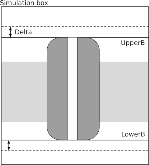
Figure flux-scheme: Scheme of the definition of upper boundary, lower boundary and delta in the case of a membrane protein.

Options:

Option | Type | Description | Default
-----|-----|-----
--TITLE | string | a title, used as output file name | flux
--SELE | string | Selection for the tracked atoms | \verb#///OH2#
--LOWER | float | Lower boundary | No default
--UPPER | float | Upper boundary | No default
--DELTA | float | Delta for the two boundaries | 5~\AA
--REF | string | Atoms selection for the channel | \verb#///CA#
--RCUT | float | Radius of the cylinder in which the transition are taken into account | Not used

As usual, --TITLE species a title for the run, while --SELE defines which atoms are tracked along the trajectory; thus if a flux of chlorine ions is wanted --SELE should contain something like ///CL, while if a water flux is needed the default (///OH2) can be used. As a side note, only one atom per tracked molecule has to be selected, so for water only the oxygen atoms are selected. The --TITLE is used as base for an output file called title-trans.dat#, which contains all the spotted transitions.

The two options --LOWER and --UPPER have been already described, together with --DELTA#, which was created to avoid PBC issues. Indeed, working with PBC, one has to take care of not counting false transition events of water molecules, i.e.\ from the upper part of the box to the lower part of the box through the PBC. To account only for real transitions we define a thin layer of the simulation box (as shown on Fig.~\ref{fig:flux-scheme}) using the upper or lower boundary and a delta value set by default to 5~\AA. All molecules over --UPPER plus --DELTA or below --LOWER minus --DELTA are given the undefined status~3.

The --REF and --RCUT options were designed so one can be sure the transition spotted occurs inside the channel and not outside of it. A transition is spotted only if the molecule pass thought the channel staying inside a vertical cylinder centered at the center the channel and having radius --RCUT#. The --REF keyword specifies which atoms build the channel, so to define its center. This option can be used, for instance, to remove the few events of transition that could happen through the lipid bilayer in the case of a protein channel embedded in membrane. By default, this option is disabled.

Sample Input:

# file flux.winp
BEGIN FLUX
--SELE /*/*/OH2
--LOWER -50.83
--UPPER 2.432
--DELTA 5.0
--RCUT 15.0
END

Sample Command Line:

wordom -iA flux.inp -imol mol.pdb -itrj traj.dcd -otxt output.out

---

Curvature (CURVATURE)

This function estimates the mean and Gaussian curvatures of a set of atoms by least-square fitting a quadratic surface over them. This can notably be useful to measure the global twist of a β-sheet. The approach is inspired by ⁴⁰ although our conventions are slightly different. The defining equation of a quadratic surface reads:

The parameters p₀, ..., p₅ are fitted on the --SELE atomic coordinates using the Levenberg-Marquardt algorithm implemented in the levmar library ⁴¹,⁴². The algorithm minimizes the quadratic error

The local curvatures of a surface are computed from its hessian matrix H. In the case of a quadratic surface, the hessian is constant and reads:

The mean curvature μ and the gaussian curvature Γ are defined as follows:

See figure curvature for a visual illustration.

By default, the curvature function returns the mean curvature mean, the gaussian curvature gaussian and the root mean square residual error error, such that:

Other interesting quantities are the two principal curvatures κ₁ and κ₂ defined as the eigenvalues of H. One has from elementary linear algebra:

The eigenvectors of the hessian matrix define two principal directions of curvature. The eigenvalues κ₁ and κ₂ give the curvature radius in the associated principal directions.

Sample Input:

# file curvature.winp
BEGIN curvature
-- TITLE A
-- SELE / A / @ (138 -148|181 -190|201 -211)/ CA
END

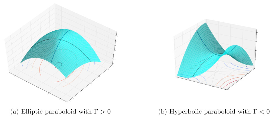
Some types of quadratic surfaces. The black lines show the principal directions of curvature.

---

More Analyses

Some analysis do not require mol or trj files, being run on different data (possibly obtained by processing mol/trj files). These modules are called using the -ie/-iE flags, rather than -ia/-iA (uppercase for input file, lowercase for command line)

---

Free Energy Profiles (FEP)

For the theory behind this, check the pdf manual the wordom paper and ²².

---

Pfold

Options:

Flag	Argument	Input	Default
-ie/BEGIN	pfoldf	call this module
--CLUSFILE	string	timeseries of noderanks
--TEMP	float	temperature of the system	300K
--LAMBDA	float	Lagrange multiplier	0.0001 (if target2=0); 0(else)
--TARGET	string	start node (pfold = 1)
--TARGET2	string	stop node (node with pfold=0)	0 (=extra node)
--NIT	int	# of iterations to solve the equations	50000
--SYMM	force symmetrization of network	no argument
--NONSYMM	prevents symmetrization of network	no argument

Note that the output file contains nodes sorted according to their weight (number of snapshots). Therefore, to plot the profile it is possible to stop the calculation after a desired number of output pairs and then sort according to column 1 (e.g.,

sort -nk1). The columns in the output file are $1=ZA /Z, $2=∆G,

$3=_p_fold , $4=rank of node

By default a non-symmetrized (detailed balance is not imposed) network is used: you can force detailed balance by specifying the --SYMM option.

ATTENTION: If pieces of trajectories from different simulations are concatenated, insert a line with the entry “0” in between to prevent spurious transitions, i.e., to avoid them to be treated as a continous timeseries. “0” must not be used otherwise.

Sample Command Line:

wordom -ie pfoldf --CLUSFILE noderank.tt --TARGET 1 --TARGET2 0 --LAMBDA 0.0001 --NIT 100000

Pfoldfnet

Instead of reading the timeseries of the noderanks, it is also possible to calculate the profile from the linkfile (i.e., the network). Note that this is more efficient than using the option --CLUSFILE.

Options:

Flag	Argument	Input	Default
-ie/BEGIN	pfoldfnet	call this module
--LINKFILE	string	links and weights (three-column file)
--TEMP	float	temperature of the system	300K
--LAMBDA	float	Lagrange multiplier	0.0001 (if target2=0); 0(else)
--TARGET	string	start node (pfold = 1)
--TARGET2	string	stop node (node with pfold=0)	0 (=extra node)
--NIT	int	# of iterations to solve the equations	50000
--SYMM	force symmetrization of network	no argument
--NONSYMM	prevents symmetrization of network (default)	no argument

The output format is identical to the one from the pfoldf function.

Sample Command Line:

wordom -ie pfoldfnet --LINKFILE linkfile.txt --TARGET 1 --TARGET2 0 --LAMBDA 0.0001

Mean First Passage Time (mfpt)

Options:

Flag	Argument	Input	Default
-ie/BEGIN	mfpt	call this module
--CLUSFILE	string	timeseries of noderanks
--TEMP	float	temperature of the system	300K
--TARGET	string	start node (pfold = 1)
--NIT	int	# of iterations to solve the equations	50000
--SYMM	force symmetrization of network	no argument
--NONSYMM	prevents symmetrization of network (default)	no argument

As for pfoldf, the output file contains nodes sorted according to their weight (number of snapshots). Therefore, to plot the profile it is possible to stop the calculation after a desired number of output pairs and then sort according to column 1 (e.g.,

sort -nk1). To use mfpt as reaction coordinate instead of ZA /Z:

the columns in the output file are $1=ZA /Z, $2=∆G, $3=mfpt, $4=rank of node. Therefore, (x=$1,y=$2) is the usual ∆G vs. ZA /Z plot, while (x=$3, y=$2) is the ∆G vs. mfpt plot, where the separation from the target basin is measured by a distance in time units.

By default a non-symmetrized (detailed balance is not imposed) network is used: you can force detailed balance by specifying the --SYMM option.

ATTENTION: If pieces of trajectories from different simulations are concatenated, insert a line with the entry “0” in between to prevent spurious transitions, i.e., to avoid them to be treated as a continous timeseries. “0” must not be used otherwise.

Sample Command Line:

wordom -ie mfpt --CLUSFILE noderank.tt --TARGET 1 --NONSYMM --TEMP 330

Mfptnet

In analogy to the pfoldfnet function, also mfpt profiles can be calculated by giving the linkfile as input. This is more efficient than using the clusfile.

Options:

Flag | Argument | Input | Default
-ie/BEGIN | mfptnet | call this module |
--LINKFILE | string | links and weights (three-columns file) |
--TEMP | float | temperature of the system | 300K
--TARGET | string | start node (pfold = 1) |
--NIT | int | # of iterations to solve the equations | 50000
--SYMM | | prevents symmetrization of network | no argument
--NONSYMM | | | prevents symmetrization of network (default) | no argument

Sample Command Line:

wordom -ie mfptnet --LINKFILE linkfile.txt --TARGET 1 --TEMP 330

A posteriori equilibration of out of equilibrium simulations

See manual for details

Options:

Flag	Argument	Input	Default
-ie/BEGIN	equil	call this module
--LINKFILE	string	links and weights (three-columns file)
--NIT	int	# of iterations to solve the equations	100000

Sample Command Line:

wordom -ie equil --LINKFILE linkfile.txt --NIT 80000

---

Kinetic Grouping Analysis(KGA)

For the theory behind this, check the pdf manual the wordom paper and ²³.

---

logbin module:First passage time plot to find τcommit

Reads in the timeseries of noderanks (i.e., a one-column file, each row indicating the rank of the population of the node, e.g., most populated node=1, second most populated node=2, etc.) and gives back the x- and y-coordinates of the logarithmically binned free-energy fpt-plot with respect to a selected node.

Options:

Flag	Argument	Input
-ie/BEGIN	logbin	option to call the logbin module
--CLUSFILE	string	timeseries of noderanks
--BPD	int	bins per decade
--TARGET	int	nodename with respect to which the first passage time should be calculated

Sample Command Line:

wordom -ie logbin --CLUSFILE noderank.tt --BPD 10 --TARGET 1

ka module: Kinetic grouping analysis to isolate all basins at once

Reads in the timeseries of noderanks and groups nodes into basins according to KGA. The procedure calculates the all-against-all matrix for a selected number of most populated nodes and assigns all other nodes in a postprocessing step.

Options:

Flag	Argument	Input
-ie/BEGIN	ka	option to call the kga module
--CLUSFILE	string	timeseries of noderanks
--TCOMM	int	commitment time τcommit (number of frames)
--NNODES	int	number of nodes for all-against-all

Sample Command Line:

wordom -ie ka --CLUSFILE noderank.tt --TCOMM 50 --NNODES 500

basin module: Kinetic grouping analysis to isolate a single basin

Reads in the timeseries of noderanks. The output is the list of commitment probabilities (_p_commit ) of all nodes to the target node. The last part of the output is a list of all nodes in the basin of the selected targetnode.

Options:

Flag	Argument	Input
-ie/BEGIN	basin	option to call the basin isolation module
--CLUSFILE	string	timeseries of noderanks
--TCOMM	int	commitment time τcommit (number of frames)
--TARGET	int	nodename (rank) of the target node

Sample Command Line:

wordom -ie basin --CLUSFILE noderank.tt --TCOMM 50 --TARGET 1

---

Invariant Core (invcore)

This method can be used to identify the most invariant region of a protein structure in a molecular dynamics simulation²⁹.

Options:

Option	Type	Description
--TITLE	string	used as output file name.
--MOLECULE	string	a molecule file.
--TRAJECTORY	string	a trajectory file.
--SELE	selection string	the invariant core will be calculated on these atoms.
--WRITEDCD	yes or no	if yes, a new trajectory file is written with the aligned frames.
--WRITEAVG	yes or no	if yes, writes the average structure calculated over aligned frames.
--MODE	string	valid values are: volume, rmsf (see below).
--STOPRULE	string	valid values are: value, value%, atoms, atoms% (see below).
--STOPVALUE	float	halts the invariant core calculation when this value is reached.

The invariant core is found using an iterative multi-step algorithm that can be summarized as follows: 1) At the beginning, all atoms are considered to be a member of the putative invariant core. 2) All atoms in the putative invariant core are used to superimpose all trajectory frames on the average structure obtained in the previous cycle (see point 4) or on the first frame in the first iteration. 3) The mobility of each atom is assessed and the atom with the highest mobility is removed from the pool of atoms of the putative invariant core. 4) An average structure is calculated after superimposing all trajectory frames using all but the most mobile atom identified in step 3. 5) Return to step 2.

This option sets the criterion to select the atom with the highest mobility in each iteration. If this option is set to volume, the mobility of each atom is expressed in terms of the volume of an error ellipsoid whose orientation and axes lengths are calculated from the eigenvalues obtained by diagonalizing the variance-covariance matrix of its coordinates. If this option is set to volume, the atom with the highest volume will be discarded from the invariant core at each iteration. On the other hand, if this option is set to rmsf, the atom with the highest RMSF will be discarded from the invariant core at each iteration.

--STOPRULE and --STOPVALUE options set the rule according to which and the value at which the calculation of the invariant core will be halted if --WRITEAVG and/or --WRITEDCD option(s) is/are set to yes. The following table summarizes the use of these options:

--STOPRULE	Stop When
value	the highest volume/rmsf is ≤ than --STOPVALUE.
value%	as above, but --STOPVALUE is considered as % of the highest volume/rmsf in the first iteration.
atoms	a number of atoms equal to --STOPVALUE have been discarded.
atoms%	a % of atoms equal to --STOPVALUE have been discarded.

Sample Input:

# file invcore.winp
BEGIN invcore
--TITLE      rmsf
--SELE       /*/*/*
--MOLECULE   protein.pdb
--TRAJECTORY protein.dcd
--MODE       rmsf
--STOPRULE   value
--STOPVALUE  1.5
--WRITEAVG   yes
--WRITEDCD   yes
END

Sample Command Line:

wordom -iE invcore.winp

---

Functional Mode Analysis (fma)

Functional Mode Analysis (FMA) is a powerful analysis method that provides a link between protein function and dynamics by finding possible correlations between the essential dynamics extracted from a molecular dynamics simulation and the time series of a structural or functional descriptor calculated on the same trajectory³⁰. FMA quantifies the contributions of individual principal components to the fluctuations of the structural/functional descriptor and, by using the Pearson coefficient, finds the linear combination of principal components that are maximally correlated with it.

This analysis is not a time series, several text and PDB output files will be created as output.

Options:

Option	Type	Description
--TITLE	string	used to generate the name of output files.
--DESCFILE	string	file name of the functional descriptor.
--DESCCOL	integer	column number of the functional descriptor present in --DESCFILE.
--PROJFILE	string	file with PCA projections generated by Wordom PRJ module.
--FIRSTPROJ	integer	first projection to load from file --PROJFILE.
--LASTPROJ	integer	last projection to load from file --PROJFILE.
--EIGVECFILE	string	file with PCA eigenvectors generated by Wordom PCA module.
--FIRSTMODELFRAME	integer	together with --LASTMODELFRAME, defines the range of the original trajectory to be used to construct the model.
--LASTMODELFRAME	integer	together with --FIRSTMODELFRAME, defines the range of the original trajectory to be used to construct the model.
--FIRSTMODELFRAME	integer	together with --LASTTESTFRAME, defines the range of the original trajectory to be used to test the model.
--LASTMODELFRAME	integer	together with --FIRSTTESTFRAME, defines the range of the original trajectory to be used to test the model.
--REFMOLFILE	string	a PDB file, used to generate multimodel pdb files.
--SELE	selection string	the very same selection used in PCA calculation.
--NUMOFMOVIEFRAMES	integer	number of models in the output multimodel PDB output file.

Sample Input:

# file fma.winp
BEGIN fma
--TITLE            fma
--DESCFILE         some_descriptors.txt
--DESCCOL          2
--PROJFILE         protein_prj.dat
--FIRSTPROJ        1
--LASTPROJ         500
--EIGVECFILE       protein-eigvec.txt
--FIRSTMODELFRAME  1
--LASTMODELFRAME   50000
--FIRSTTESTFRAME   50001
--LASTTESTFRAME    100001
--REFMOLFILE       protein.pdb
--SELE             /*/*/*
--NUMOFMOVIEFRAMES 30
END

Sample Command Line:

wordom -iE fma.winp

FMA is a complex analysis and this module generates several output files.

File Name	Description
fma_test-info.txt	a text file with a detailed a description of each output file.
fma_test-contr.dat	a four columns table with the (cumulative) contribution of each vector in explaining the functional descriptor and the percentage of their explained variance.
fma_test-ewmcm-eigvec.txt	a text file with the eigenvector of the ensemble-weighted maximally correlated motion.
fma_test-ewmcm.pdb	a multi-model PDB file with ensemble-weighted maximally correlated motion.
fma_test-mcm-eigvec.txt	a text file with the eigenvector of the maximally correlated motion.
fma_test-pear_nev.dat	a three columns table with the correlation between the model/validation set and the functional descriptor as a function of the number of eigenvectors.
fma_test-sig_nev.dat	similar to the file above but with the residuals of data and models.
fma_test-validate_desc_vs_model.dat	a three columns table with the real and predicted value of the functional descriptor as a function of each trajectory frame in the range defined by --FIRSTMODELFRAME and --LASTMODELFRAME options.
fma_test-validate_desc_vs_valid.dat	a three columns table with the real and predicted value of the functional descriptor as a function of each trajectory frame in the range defined by --FIRSTTESTFRAME and --LASTTESTFRAME options.

---

Clustering based on Correlation Of Atomic Fluctuation (corrclust)

With this module is possible to cluster atoms/residues based on the pairwise correlation of their atomic fluctuations. Atoms are assigned to a cluster using an agglomerative hierarchical algorithm based on four possible well-known distance measures: Average, Complete, Single, and Ward.

This module can be used to find dynamic protein domains that move as coherent units in a simulation as proposed in the method named Geometrically Stable Substructures (GeoStaS)³⁴. Wordom not only retains all the features of the original method but extends it by allowing the use of any of the four available algorithms for calculating the correlations of atomic fluctuations from molecular dynamic simulations (i.e. DCC, LMI, DiCC, and AMS), as well as the correlations derived from ENM-NMA, thus making the method applicable also to a single structure.

Options:

Option	Type	Description
--TITLE	string	used to generate the name of output files.
--K	integer	number of desired clusters, see below.
--MATRIX	string	the output file of Wordom Corr module.
--MOLFILE	string	a PDB file, see below.
--METHOD	string	name of the distance measure to use, valid values are: average, complete, single, and ward.
--CALCDIST	yes or no	set to yes if the file passed to --MATRIX is has correlation values and then the distances must be calculated.

--K option is used to set the desired number of clusters, if 0 is passed, the number of clusters will be automatically chosen using the Silhouette Index method³⁵.

Sample Input:

# file corrclust.winp
BEGIN corrclust
--TITLE    corrclust
--K        0
--METHOD   average
--MATRIX   protein.lmi
--MOLFILE  protein.pdb
--CALCDIST yes
END

Sample Command Line:

wordom -iE corrclust.winp

This module generates three output files named after the string passed to --TITLE option. A file with .txt extension with the cluster of each atom/residue, a PDB file with the cluster of each atom in the β-factor field and a .log extension with some info about the clustering process.

---

PCA Tools (pcatools)

This module performs several useful post-analyses on the outputs of PCA and ENM-NMA modules. With this module, it is possible to compute the dot product of any number of pairs of eigenvectors, the overlap between an eigenvector and a deformation vector, and the cumulative squared overlap between two sets of eigenvectors.

Options:

Option	Type	Description
--TITLE	string	used to generate the name of output files.
--EVFILE1	string	the name of a Wordom eigenvector file.
--EVFILE2	string	the name of a Wordom eigenvector file.
--EVRANGE1	two integers	the first and the last eigenvector to load from the file passed to --EVFILE1.
--EVRANGE2	two integers	the first and the last eigenvector to load from the file passed to --EVFILE2.
--CALC	string	either EVEVOVERLAP or EVDVOVERLAP, see below.
--RMSD	float	used only if --CALC is set to EVDVOVERLAP, see below.
--FITTEDATOMS	integer	used only if --CALC is set to EVDVOVERLAP, see below.

If --CALC option is set to EVEVOVERLAP, Wordom will calculate the dot products between pairs of eigenvectors selected with --EVRANGE1 and --EVRANGE2 options. If this option is set to EVDVOVERLAP, Wordom will compute the overlap between an eigenvector and a deformation vector. In this case, the RMSD value between the two conformation and the number of atoms used to calculate this value must be provided using the --RMSD and --FITTEDATOMS options.

Sample Input:

# file pcatools.winp
BEGIN pcatools
--TITLE pcatools
--EVFILE1 protein_wt-eigvec.txt
--EVFILE2 protein_mut-eigvec.txt
--EVRANGE1 1 5
--EVRANGE1 1 3
--CALC EVEVOVERLAP
END

Sample Command Line:

wordom -iE pcatools.winp

With the example input above, Wordom will produce the following 4 output files:

File Name	Description
pcatools-pcaoverlap.log	a file with a summary of performed calculations.
pcatools-overlap_matrix.dat	a matrix with the dot products between the first 5 eigenvectors from file protein_wt-eigvec.txt and the first 3 eigenvectors from file protein_mutt-eigvec.txt.
pcatools-cso_1vs2.dat	the cumulative square overlap between selected eigenvectors.
pcatools-cso_2vs1.dat	the cumulative square overlap between selected eigenvectors.

---

Perturbation Response Scanning (prs)

PRS²⁴ is a powerful technique that can assess and quantify the importance of each protein residue in determining conformational changes as a consequence of external perturbations. Over time, the method has been subjected to several developments and expansions²⁷, ²⁶, ²⁸, all included in this version of Word. In particular, given two conformations of the same protein, an initial and a target structure, PRS can predict protein residues that, under the influence of external perturbations, cause a conformational change closest to the target structure. Additionally, this method is also able to identify and quantitatively assess the effectiveness and sensitivity of each protein residue, i.e. the ability of a given residue in transmitting signals when subjected to a perturbation and the ability of a residue to detect signals transmitted by effectors, respectively. PRS, which is based on the Linear Response Theory³¹, can be used to analyze both single structures and molecular dynamics simulations. PRS relies on systematically applying virtual random forces on each protein residue and detecting the linear response of the whole protein to these perturbations.

Options:

Option	Type	Description
--TITLE	string	used to generate the name of output files.
--COVMAT	string	file name of the covariance matrix. The format is the same produced by Wordom PCA and ENM modules.
--TESTMOL	string	a PDB file name, used to generates PDB output files.
--PERTNUM	integer	set the number of random forces to be applied.
--SAMEFORCES	yes or no	if yes, apply the same set of random forces to all atoms.
--LOADPERT	string	a file name, can be used to load and apply the same set of random forces to different systems/runs.
--CUTOFF	float	option used to set the minimum significance value of sensitivity and specificity. If set to -1, the average sensitivity and specificity will be used.
--DCISELE	string + selection string	can be present more than once, used to assign a name and to select atoms for Dynamic Coupling Index (DCI) analysis.
Sample Input:

# file prs.winp
BEGIN prs
--TITLE prs
--COVMAT protein-matrix.txt
--TESTMOL protein.pdb
--PERTNUM 0
--CUTOFF 50
END

Sample Command Line:

wordom -iE prs.winp

With the example input above, Wordom will produce the following output files:

File Name	Description
prs-summary.log	a summary text file with used options and a table with the effectiveness and sensitivity values above the threshold passed to --CUTOFF option.
prs.pdb	A PDB file with the effectiveness and sensitivity value of each residue saved in the β factor and occupancy field, respectively.
prs_test-response_matrix.txt	a text file with the response matrix organized by row.
prs_test-effectiveness.txt	a table with the effectiveness value of each residue.
prs_test-sensitivity.txt	a table with the sensitivity value of each residue.
prs_test-dci_residues.txt	a table with the dynamic coupling index of each residue.
prs_test-dfi_residues.txt	a table with the dynamic flexibility index of each residue.

---

References

Seeber 2007: M. Seeber, M. Cecchini, F. Rao, G. Settanni, and A. Caflisch, Bioinformatics, 2007, 23(19), 2625–2627.
Seeber 2011: M. Seeber, A. Felline, F. Raimondi, S. Muff, R. Friedman, F. Rao, A. Caflisch, and F. Fanelli, J. Comp. Chem, 2010, in press.

---

1. M. Seeber, M. Cecchini, F. Rao, G. Settanni, and A. Caflisch, Bioinformatics, 2007, 23(19), 2625–2627. ↩

2. M. Seeber, A. Felline, F. Raimondi, S. Muff, R. Friedman, F. Rao, A. Caflisch, and F. Fanelli, J. Comp. Chem, 2011, 6(32):1183-1194 ↩

3. M. Cecchini, F. Rao, M. Seeber, and A. Caflisch, J. Chem. Phys., 2004, 121. ↩

4. I. Andricioaei and M. Karplus, J. Chem. Phys., 2001, 115, 6289–6292. ↩

5. W. Kabsch and C. Sander, Biopolymers, 1983, 22(12), 2577–637. ↩

6. C. A. F. Andersen, A. G. Palmer, S. Brunak, and B. Rost, Structure, 2002, 10, 174–184. ↩

7. P. Carter, C.A.F. Andersen, and B. Rost, Nucleic Acids Research, 2003, 31(13), 3293. ↩

8. Tirion, M., Phys Rev Lett, 1996, 77(9), 1905–1908. ↩

9. Delarue, M. and Sanejouand, Y., J Mol Biol, 2002, 320(5), 1011–1024. ↩

10. Kovacs, J.; Chacon, P. and Abagyan, R., Proteins, 2004, 56(4), 661–668. ↩

11. Durand, P.; Trinquier, G.; Sanejouand, Y.-H., Biopolymers 1994, 34, 759−771. ↩

12. Tama, F.; Gadea, F. X.; Marques, O.; Sanejouand, Y. H., Proteins 2000, 41, 1−7 ↩

13. Zheng, W.; Brooks, B. R, Biophys. J. 2005, 89, 167−178. ↩

14. Zheng,W.; Brooks, B.; Doniach, S.; Thirumalai, D. Structure 2005, 13,565. ↩

15. Wang, Y.; Rader, A. J.; Bahar, I.; Jernigan, R. L, J. Struct. Biol. 2004, 147, 302−314.
    [^Busa 2005] J. Busa, J. Dzurina, E. Hayryan, S. Hayryan, C.K. Hu, J. Plavka, I. Pokorny, J. Skrivrnek, and M.C. Wu, Computer Physics Communications, 2005, 165(1), 59–96. ↩

16. JL Pascual-Ahuir, E. Silla, and I. Tunon, Journal of Computational Chemistry, 1994, 15(10). ↩

17. J.A. McCammon and S.C. Harvey, Dynamics of proteins and nucleic acids; Cambridge Univ Pr, 1988. ↩↩

18. A. Kraskov, H. Stoegbauer, and P. Grassberger, Physical Review E, 2004, 69(6), 66138. ↩↩

19. O.F. Lange and H. Grubmuller, PROTEINS-NEW YORK-, 2006, 62(4), 1053. ↩↩

20. K.V. Brinda, S. Vishveshwara, A network representation of protein structures: implications for protein stability, Biophys J, 89 (6) (2005), pp. 4159-4170 ↩

21. A. Ghosh and S. Vishveshwara, Proceedings of the National Academy of Sciences, 2007, 104(40), 15711. ↩

22. S. V. Krivov and M. Karplus, J. Phys. Chem. B, 2006, 110, 2689–12698. ↩

23. S. Muff and A. Caflisch, Proteins: Structure, Function, and Bioinformatics, 2008, 70, 1185–1195. ↩

24. Atilgan C, Atilgan AR (2009) Perturbation-Response Scanning Reveals Ligand Entry-Exit Mechanisms of Ferric Binding Protein. PLoS Comput
    Biol 5(10): e1000544. doi:10.1371/journal.pcbi.1000544 ↩

25. Benson, N. C.; Daggett, V. Wavelet Analysis of Protein Motion. Int. J. Wavelets Multiresolut. Inf. Process 2012, 10, 1250040 ↩

26. Campitelli, P.; Ozkan, S.B. Allostery and Epistasis: Emergent Properties of Anisotropic Networks. Entropy 2020, 22, 667. https://doi.org/10.3390/e22060667 ↩

27. Dutta A, Krieger J, Lee JY, Garcia-Nafria J, Greger IH, Bahar I. Cooperative Dynamics of Intact AMPA and NMDA Glutamate Receptors: Similarities and Subfamily-Specific Differences. Structure. 2015;23(9):1692-1704. doi:10.1016/j.str.2015.07.002 ↩

28. Nevin Gerek Z, Kumar S, Banu Ozkan S. Structural dynamics flexibility informs function and evolution at a proteome scale. Evol Appl. 2013 Apr;6(3):423-33. doi: 10.1111/eva.12052. Epub 2013 Feb 13. PMID: 23745135; PMCID: PMC3673471. ↩

29. Gerstein M, Altman RB. Average core structures and variability measures for protein families: application to the immunoglobulins. J Mol Biol. 1995;251(1):161-175. doi:10.1006/jmbi.1995.0423 ↩

30. Hub JS, de Groot BL (2009) Detection of Functional Modes in Protein Dynamics. PLOS Computational Biology 5(8): e1000480. doi.org/10.1371/journal.pcbi.1000480 ↩

31. Ikeguchi M, Ueno J, Sato M, Kidera A (2005) Protein structural change upon ligand binding: linear response theory. Phys Rev Lett 94: 078102. ↩

32. Levine BG, Stone JE, Kohlmeyer A. Fast Analysis of Molecular Dynamics Trajectories with Graphics Processing Units-Radial Distribution Function Histogramming. J Comput Phys. 2011 May 1;230(9):3556-3569. doi: 10.1016/j.jcp.2011.01.048 ↩

33. Münz M, Hein J, Biggin PC (2012) The Role of Flexibility and Conformational Selection in the Binding Promiscuity of PDZ Domains. PLOS Computational Biology 8(11): e1002749. https://doi.org/10.1371/journal.pcbi.1002749 ↩

34. Julia Romanowska, Krzysztof S. Nowiński, and Joanna Trylska, Determining Geometrically Stable Domains in Molecular Conformation Sets, Journal of Chemical Theory and Computation 2012 8 (8), 2588-2599 DOI: 10.1021/ct300206j ↩↩

35. Peter J. Rousseeuw, Silhouettes: A graphical aid to the interpretation and validation of cluster analysis, Journal of Computational and Applied Mathematics, 20, 1987, 53-65, doi.org/10.1016/0377-0427(87)90125-7. ↩

36. Roy A, Hua DP, Post CB. Analysis of Multidomain Protein Dynamics. J Chem Theory Comput. 2016;12(1):274-280. doi:10.1021/acs.jctc.5b00796 ↩

37. Sacquin-Mora, S., Laforet, É. and Lavery, R. (2007), Locating the active sites of enzymes using mechanical properties. Proteins, 67: 350-359. https://doi.org/10.1002/prot.21353 ↩

38. Szekely, G.J., Rizzo, M.L., and Bakirov, N.K. (2007), Measuring and Testing Dependence by Correlation of Distances, Annals of Statistics, Vol. 35 No. 6, pp. 2769-2794. doi: 10.1214/009053607000000505 ↩

39. Torrence, C.; Compo, G. P. A practical guide to wavelet analysis. Bull. Am. Meteorol. Soc. 1998, 79, 61−78 ↩

40. S. Sun, D. Chandler, A. R. Dinner, G. Oster, {\em European Biophysics Journal}, {\bf 2003}, {\em 32}, 676--683. ↩

41. M. I. A. Lourakis, {\em Foundation of Research and Technology}, {\bf 2005}, {\em 4}, 1--6. ↩

42. M.I.A. Lourakis, {\em levmar: Levenberg-Marquardt nonlinear least squares algorithms in {C}/{C}++}. Available at: http://www.ics.forth.gr/~lourakis/levmar/ ↩