JANPA Wiki
Status: Beta
Brought to you by:
timn2
This page presents an example of using LPO/CLPO methods of JANPA to investigate covalent bonding in cyanamide (IUPAC name aminoformonitrile). The structural formula of the molecule is shown below:
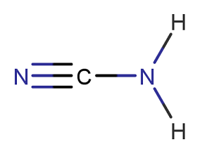
It is worth noting that each nitrogen atom typically possesses a so-called 'lone pair' (also callen 'nonbonding electron pair') commonly designated with two dots:

Above all, we need to obtain the 3D geometry of the molecule. This can be done, for example, by DFT geometry
optimization in ORCA
%MaxCore 2000
%pal nprocs 4
end

! B3LYP/G D3BJ def2-TZVP TightOpt VeryTightSCF Grid6 NoFinalGrid AnFreq

*xyz 0 1
 C         -1.86004        0.91959        0.08904
 N         -1.06624        2.04952        0.19646
 H         -0.26875        2.04728        0.84649
 H         -1.35291        2.93136       -0.25214
 N         -2.52195       -0.02688        0.00501
*
In this example we used B3LYP-D3/def2-TZVP level of theory to obtain the optimized geometry of the molecule and compute its normal vibration frequencies to ensure that the optimized geometry is stable (not a transition state). The ORCA results for this input is available for download.
The optimized geometry of the molecule looks like this:
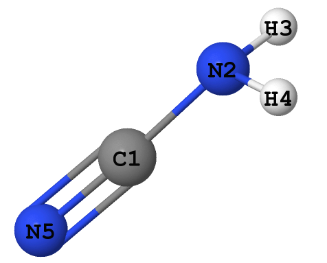
(note that this visualization uses XYZ Cartesian coordinates of the atoms as the only source of information.
Therefore, it is of no importance whether or not any of the 'sticks' are drawn between the atoms, as well as the number of these 'sticks'. In contrast to that, the bonding analysis involving the localized orbotals performed below does have a relation
to the true pattern of covalent bonding)
Note however, that we do not recommended using the 'orbitals' produced by DFT calculations for bonding analysis -
because it is a feature of the most commonly used Kohn-Sham formulation of DFT that these orbitals correspond to an
artifician 'non-interacting' system, instead of the true system.
Recall that it is the electron density, not the wavefunction* which can be obtained by DFT ! *
In order to generate the true orbitals for subsequent localization we can use MP2 method.
The following example presents the input file for PSI4 (version 1.2) and uses the optimized geometry from the previous run
memory 4200 mb

molecule struct {
 symmetry c1
 no_com
 0 1
  C   -1.82066662989926      0.95269342902260      0.07890156818907
  N   -0.98388162068735      1.99809656426149      0.07905823857676
  H   -0.35596894246243      2.05392589300360      0.86735797022724
  H   -1.39303288068047      2.88424548594471     -0.17811773761250
  N   -2.51633992627050      0.03190862776760      0.03765996061943
}

set  {
  basis       def2-tzvpp
  MOLDEN_WRITE false # set tu true if the Haftree-Fock SCF orbitals are to be analyzed as well
}

e, wfn = properties('mp2', return_wfn=True)

d = wfn.Da().to_array()
s = wfn.S().to_array()
c = wfn.Ca().to_array()
occs = c.T.dot(s.dot(d).dot(s).dot(c))

molden(wfn, 'mp2.molden', density_a = psi4.core.Matrix.from_array(occs))
For more information on the structure of this file, see using Janpa with PSI4
In this example we used MP2(full)/def2-TZVPP level of theory to produce relaxed density matrix and save it as mp2.molden file, which can be easily converted to a format appropriate for JANPA input (see below). The PSI4 results for this input is available for download. Alternatively, the natural MP2 orbitals corresponding to a relaxed density can be produced with ORCA as well. However, PSI4 is capable of being generalizable to other correlated methods (like CCSD) more straightforwardly, and tharefore was considered to be more appropriate for illustrative purposes here.
We now need to convert the mp2.molden file into the correct MOLDEN format. This can be done by a molden2molden program from Janpa package by running a command
java -jar molden2molden.jar -i mp2.molden -o input.molden -normalizebf
To analyze the electronic structure of the molecule with JANPA we now run
java -jar janpa.jar -i input.molden -CLPO_Molden_File CLPO.molden > janpa.log
This will produce two files: janpa.log containing the general output of the program and CLPO.molden suitable
for orbitals visualization with JMOL.
Note:
i) there was -ignorefock option in JANPA versions prior to 2.02. Using this option was highly recommended for analyzing the orbitals obtained from a correlated wavefunction, since in this case no 'energies' of the orbitals are available. For the same reason the default behaviour has been changed in JANPA v. 2.02, so that the Fock matrix is ignored by default. In case if for some reason the Fock matrix analysis is still needed, the option -doFock should be used.
ii) the CLPO.molden file is produced in a correct MOLDEN format and can readily be used for further CLPO orbital visualization.
Lets look into the most essential parts of the janpa.log log file (janpa.sourceforge.net).
The first thing we need to ensure is that there were no errors in the input file. For that we check the few last lines of the log:
0 warning(s)

Total run time: 0 min, 2.0 sec


                          * * *
The absence of warnings allows us to proceed with the analysis.
The first important portion of the output is
Final electron populations and NPA charges:

Center  Nuclear  Electron     NMB           NPA
         charge  population   population    charge
   C1       6.0   5.6107618    5.5459659     0.3892382404
   N2       7.0   7.8403209    7.7572929    -0.8403209443
   H3       1.0   0.5976361    0.5914083     0.4023638511
   H4       1.0   0.5976334    0.5914055     0.4023666271
   N5       7.0   7.3534478    7.2746655    -0.3534477746
and presents the NPA charges of the atoms.
Another portion related to bonding is
Wiberg-Mayer bond indices:
Centr. A/B         1         2         3         4         5
      1    ( 3.6447)    1.0792    0.0018    0.0018    2.5619
      2              ( 2.7513)    0.7725    0.7725    0.1270
      3                        ( 0.7944)    0.0003    0.0198
      4                                  ( 0.7944)    0.0198
      5                                            ( 2.7285)
reporting the bond orders computed accordign to K.Wiberg definition from the density matrix in NAO basis.
The most essential part of bonding analysis (actually, the CLPO analysis), however, is contained in the lines
*** Summary of CLPO results

  CLPO           D e s c r i p t i o n      Occupancy   Composition
    3                               C1 (RY)   0.00408   1.0 * h3@C1
    4   (BD) C1-N2, Io = 0.1950             1.96394     h4@C1 * ( 0.6344) + h35@N2 * ( 0.7730)
    5        C1-N2, antibonding (NB)          0.04500   h4@C1 * (-0.7730) + h35@N2 * ( 0.6344)
    6   (LP)  C1                            1.99844     1.0 * h5@C1
   10                               C1 (RY)   0.00230   1.0 * h9@C1
   11                               C1 (RY)   0.02158   1.0 * h10@C1
   12                               C1 (RY)   0.00487   1.0 * h11@C1
   13   (BD) C1-N5, Io = 0.1268             1.96923     h12@C1 * (-0.6608) + h102@N5 * ( 0.7506)
   14        C1-N5, antibonding (NB)          0.02785   h12@C1 * (-0.7506) + h102@N5 * (-0.6608)
   15   (BD) C1-N5, Io = 0.0777             1.91413     h13@C1 * ( 0.6791) + h103@N5 * ( 0.7341)
   16        C1-N5, antibonding (NB)          0.08438   h13@C1 * (-0.7341) + h103@N5 * ( 0.6791)
   17   (BD) C1-N5, Io = 0.1397             1.93044     h14@C1 * ( 0.6559) + h104@N5 * ( 0.7549)
   18        C1-N5, antibonding (NB)          0.18407   h14@C1 * (-0.7549) + h104@N5 * ( 0.6559)
   24                               C1 (RY)   0.00385   1.0 * h20@C1
   25                               C1 (RY)   0.00379   1.0 * h21@C1
   26                               C1 (RY)   0.00388   1.0 * h22@C1
   27                               C1 (RY)   0.00515   1.0 * h23@C1
   38                               N2 (RY)   0.00651   1.0 * h34@N2
   39   (LP)  N2                            1.99867     1.0 * h36@N2
   40                               N2 (RY)   0.00235   1.0 * h37@N2
   43                               N2 (RY)   0.00181   1.0 * h40@N2
   44                               N2 (RY)   0.00241   1.0 * h41@N2
   45                               N2 (RY)   0.01609   1.0 * h42@N2
   46   (BD) N2-H3, Io = 0.4098             1.94850     h43@N2 * ( 0.8396) + h65@H3 * ( 0.5432)
   47        N2-H3, antibonding (NB)          0.02417   h43@N2 * ( 0.5432) + h65@H3 * (-0.8396)
   48   (BD) N2-H4, Io = 0.4098             1.94850     h44@N2 * ( 0.8396) + h79@H4 * ( 0.5432)
   49        N2-H4, antibonding (NB)          0.02417   h44@N2 * ( 0.5432) + h79@H4 * (-0.8396)
   50   (LP)  N2                            1.82926     1.0 * h45@N2
   56                               N2 (RY)   0.00648   1.0 * h51@N2
   58                               N2 (RY)   0.00664   1.0 * h53@N2
   59                               N2 (RY)   0.00554   1.0 * h54@N2
   60                               N2 (RY)   0.00554   1.0 * h55@N2
   69                               H3 (RY)   0.00177   1.0 * h64@H3
   75                               H3 (RY)   0.00174   1.0 * h71@H3
   82                               H4 (RY)   0.00180   1.0 * h78@H4
   88                               H4 (RY)   0.00175   1.0 * h85@H4
   96                               N5 (RY)   0.01168   1.0 * h93@N5
   97   (LP)  N5                            1.93003     1.0 * h94@N5
   98   (LP)  N5                            1.99866     1.0 * h95@N5
  100                               N5 (RY)   0.00114   1.0 * h97@N5
  102                               N5 (RY)   0.00585   1.0 * h99@N5
  103                               N5 (RY)   0.00564   1.0 * h100@N5
  104                               N5 (RY)   0.00738   1.0 * h101@N5
  110                               N5 (RY)   0.00510   1.0 * h110@N5
  111                               N5 (RY)   0.00514   1.0 * h111@N5
  112                               N5 (RY)   0.00394   1.0 * h112@N5
  113                               N5 (RY)   0.00249   1.0 * h113@N5

Note: 74 one-center RY orbitals, each having occupancy below 1.00e-03,
      were not printed (use the program option -RyOccPrintThreshold to change this behavior)
      Total occupancy of these RY orbitals is 0.02212


Number of two-center(2C) orbitals for each pair of atoms
Centr. A/B         1         2         3         4         5
      1    (      4)         1         0         0         3
      2              (      3)         1         1         0
      3                        (      1)         0         0
      4                                  (      1)         0
      5                                            (      3)
VAL:      C      4
VAL:      N      3
VAL:      H      1
VAL:      H      1
VAL:      N      3

>> CLPO occupancy summary >>
       bonding (BD):     11.67473 in    6 oribtals
  anti-bonding (NB):      0.38964 in    6 oribtals
 1c-lone pairs (LP):      9.75506 in    5 oribtals
 1c-unoccupied (RY):      0.18037 in  104 oribtals

Method        BD+LP....in      NB+RY     BD+NB+LP  BD+NB+LP+RY      trace(D)   Sum[Bd^2+Lp^2]    ||D||^2
  CLPO     21.42979    11    0.57001     21.81943     21.99980       22.000        41.7730       42.6760
That means that CLPOs 4, 13, 15, 17, 46 and 48 describe the covalent bonds connecting the atoms C1-N2,
C1-N5, C1-N5, C1-N5, N2-H3 and N2-H4 respectively. In other words, there are some single bods,
and a triple bond between C1 and N5 -- in exact agreement with the structural formula of the molecule given above!
In addition to that, CLPOs 6, 39, 50, 97 and 98 are the non-bonding (or 'lone') pairs. As will be evident from the below
visualization of these orbitals, CLPOs 6, 39 and 98 correspond to the 'inner shells' (commonly denoted as 1s2), while
CLPOs 50 and 97 are the lone pairs belonging to the 'valence shells' of nitrogen atoms. This is again in agreement
with our expectations!
Finally, the total number of bonds formed by each atom of the molecule (fiven as the diagonal elements of the
Number of two-center(2C) orbitals for each pair of atoms table) agree with the well-known
chemical valencies of the H, C and N atoms constituting the molecule under study.
The CLPO.molden file generated by JANPA during the previous step can now be used to visualize the localized orbitals.
To this end, JMOL program can be used. JMOL can read MOLDEN files
produced by JANPA directly: just use the File -> Open command and choose the CLPO.molden file (janpa.sourceforge.net). One can then
proceed with orbital visualization using ContextMenu -> Surfaces -> Molecular orbitals menu.
Alternatively, the following commands can be used in JMOL console (ContextMenu -> Console) to plot orbitals:
mo list
to show the full list of the orbitals, e.g.,
..............
model 1.1;  mo 8  # energy 7.000     occupancy 6.5700006E-4 beta1a
model 1.1;  mo 7  # energy 6.000     occupancy 2.8900002E-4 beta1a
model 1.1;  mo 6  # energy 5.000     occupancy 1.998445 beta1a
model 1.1;  mo 5  # energy 4.000     occupancy 0.045001 beta1a
model 1.1;  mo 4  # energy 3.000     occupancy 1.963944 beta1a
model 1.1;  mo 3  # energy 2.000     occupancy 0.004084 beta1a
model 1.1;  mo 2  # energy 1.000     occupancy 3.3300003E-4 beta1a
model 1.1;  mo 1  # energy 0.000     occupancy 5.5999997E-5 beta1a
(note that the occupancies and the orbital numbering here is exactly the same as in the *** Summary of CLPO results
table above).
The command
mo 4
can then be used to plot the selected orbital (in this case, CLPO 4), while the mo cutoff 0.1 command can be used
to adjust the contour value to which the isosurface should correspond (the value of 0.1 a.u. was used to produce
the isosurfaces shown below).
It is also possible to use the isosurface command to plot orbitals, e.g.,
isosurface color yellow dodgerblue cutoff 0.1 resolution 15 mo 15 translucent 0.45
(some nice-looking colors combinations are [250,187,13] skyblue , [255,255,0] [102,204,255], [247,255,71] [113,168,254], [250,187,13] [185,214,248], [250,187,13] blue, darkorange skyblue). In this example the translucent 0.45 produces 'semi-transparent' isosurfaces and
can be replaced with, e.g., mesh nofill to make the 'wireframe' representation as used in the illustrations below.
For more details about these and the other orbital plotting commands, see the JMOL documentation.
| Bonding orbital | Antibonding orbital | Pair of atoms |
|---|---|---|
CLPO 4 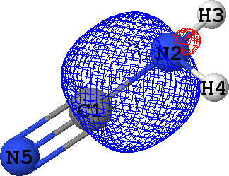 |
CLPO 5 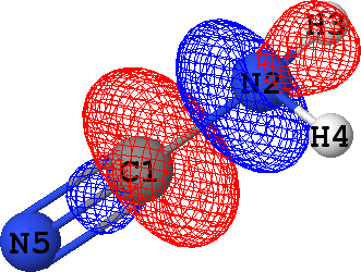 |
C1 - N2 ('sigma') |
CLPO 13 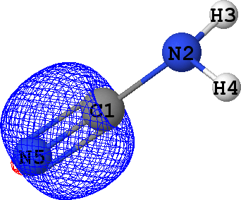 |
CLPO 14 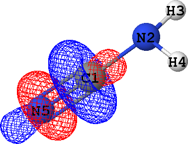 |
C1 - N5 ('sigma') |
CLPO 15 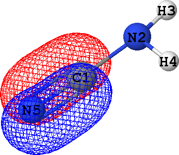 |
CLPO 16 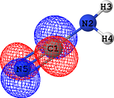 |
C1 - N5 ('first pi') |
CLPO 17 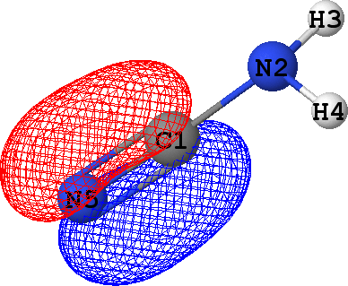 |
CLPO 18 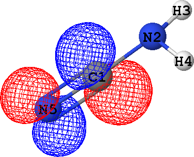 |
C1 - N5 ('second pi') |
CLPO 46 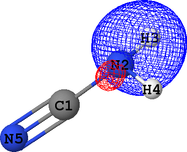 |
CLPO 47 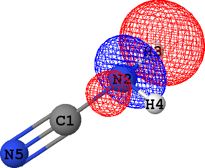 |
N2 - H3 ('sigma') |
CLPO 48 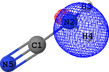 |
CLPO 49 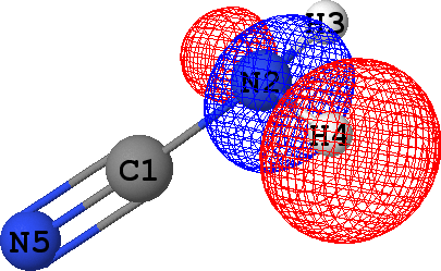 |
N2 - H4 ('sigma') |
It follows from these bonding orbital isosurfaces that each single bond anticipated from a structural formula
of the molecule is accompained by a localized bonding orbital of 'sigma' symmetry, while the triple
bond (which is usually modeled as a family of one 'sigma' and two 'pi' bonds) between N5 and C1
additionally includes two bonding orbitals of 'pi' symmetry.
Note that according to the *** Summary of CLPO results table given above, occupancies of
all bonding orbitals are very close to 2.0 (they fall in the range between 1.91 to 1.97 electrons),
which agrees with the classical Lewis picture anticipating the bond to formed by the pair of electrons.
Occupancies of antibonding orbitals are, on the other hand, quite low: mainly less than 0.1 electrons,
with the exception of CLPO 17 corresponding to one of N5-C1 'pi' bonds which has occupancy of almost 0.2 electrons
due to a possible conjugation with the lone pair of N2 (represented by CLPO 50, see below).
| Orbital | Comments |
|---|---|
CLPO 6 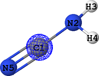 |
Core orbital of C1 |
CLPO 39 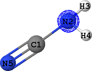 |
Core orbital of N2 |
CLPO 50 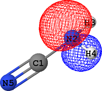 |
Lone pair of N2 |
CLPO 97 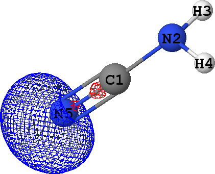 |
Lone pair of N5 |
CLPO 98 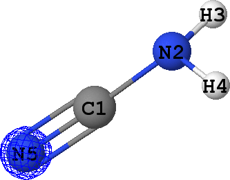 |
Core orbital of N5 |
It can be seen that there are indeed two ('valence') lone pairs, one per each of the nitrogen atoms in the molecule.
What is more, the spatial orientation of these lone pairs is in good agreement with the hybridization models
of N2 (sp3) and N5 (sp1) atoms expected from chemical intuition: the lone pair
at N5 is oriented along the same line as N5-C1 bond, while lone pair at N2 follows a 'tetrahedral' direction
along with N2-C1, N2-H3 and N2-H4 bonds.