Menu
▾
▴
* Qt installer can be downloaded from here.
* Open a terminal where the file was downloaded and run: "chmod +x 'downloaded_file_name'". Then, run: "./'downloaded_file_name'".
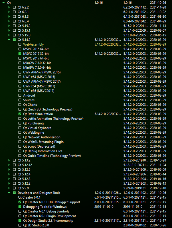
* Check the things in the Qt installer as here:
* Try to open QtCreator and load the project. If QtCreator doesn't start, run: "sudo apt-get install --reinstall qtcreator".
When opening the project for the fisrt time, you may be asked to choose a kit (the compiler for the project). In our case, we have used the GCC one: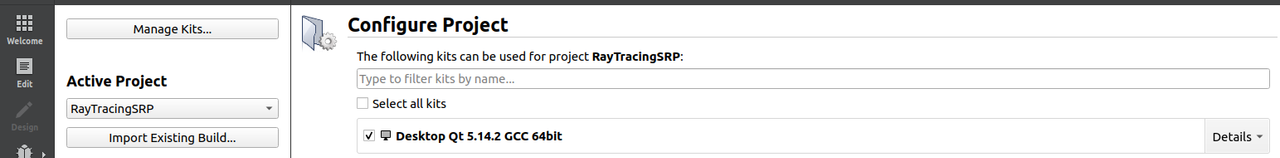
2. Install OpenGL: * Run: "sudo apt-get install libgl-dev".
* Qt installer can be downloaded from here.
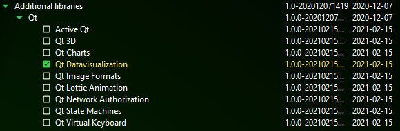
* Check the things in the Qt installer as here:

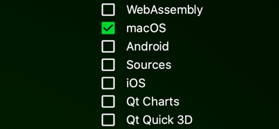
Inside the Qt version choosen (for example, "Qt 5.14.2"), enable also the macOS toggle:
When opening the project for the fisrt time, you may be asked to choose a kit (the compiler for the project). For example, you can choose the clang one: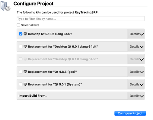
On Qt, in case you have a problem compiling the project with qmake: 1. Select the tab 'Projects' in the left side tabs. It will take you to the 'Build Settings' page.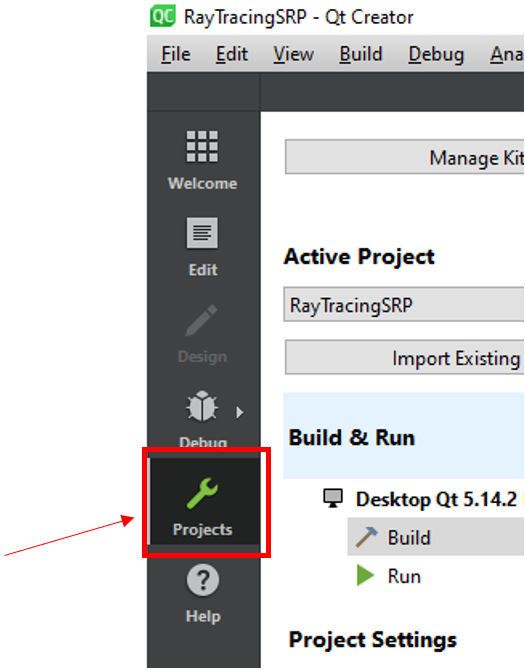
2. Add "INCLUDEPATH+=/opt/X11/include" in the qmake options: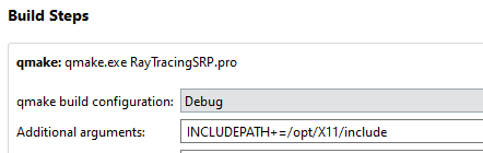
2. Install OpenGL: * Install last version of Xcode and XQuartz from the Mac AppStore.
* Check the next things when installing Visual Studio:
2. Install Qt * Qt installer can be downloaded from here.
* Check the things in the Qt installer as here:

* Try to open QtCreator and load the project. When opening the project for the fisrt time, you may be asked to choose a kit (the compiler for the project). In our case, we have used the MSCV one: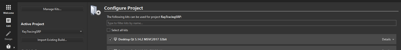
3. Regarding OpenGL: * The library of OpenGL if already in the project. However, if it requires you the file "glext.dll" or the program crashes when running the project on Qt, this dll can be found in the RayTracingSRP folder. Put this dll file in the folder where there are the compiled objects of this project.
You need to load the spacecraft model (OBJ file) which is based on CAD model: it contains the list of vertices, faces and normals (optional). Also, you need a MTL file where is described the reflectivy properties of the surface of the spacecraft. In addition, you can set its weight. In the resources/model directory there are examples of this files.
You need to choose a method (the model you want to use to approximate the SRP force):
*Cannonball (CPU): considers the shape of the spacecraft to be a sphere. Ypu can set the area of the sphere (A) and the reflectivity property (Cr).
*NPlate (CPU): considers the shape of the spacecraft to be represented as a set of flat plates (you need to load a file that contains the number of plates, and then, for each plate, a new line with the area, specular reflectivity property, diffuse reflectivity property, and normal of the plate; you can see an example in the resources/model directory).
*RayTrace (CPU): for each cell of a grid defined by the number of cells (Nx x Ny) a ray is casted against the triangular mesh of the spacecraft. Then, it is computed the SRP force on the intersected triangle. The user can set the grid and secondary and diffuse rays.
*RayTrace (GPU): Similar to the CPU version, in this case the computation is done in the GPU. The user can set the secondary and diffuse rays. (Nx = Ny = 512 by default).
You need to choose what action you want to do:
* Visualize spacecraft: when the user press the start button in the Visualize Spacecraft tab, it will show a 3D viewer of the spacecraft with its 3 axes and the sunlight direction. Then, the user can set the initial rotation of the spacecraft by interacting with the three sliders. Each one of them corresponds to one of the local axes of the spacecraft.
For example, in the first slider, it appears "X" in red and this indicates that the red line in the 3D viewer correspond to the x axis. The user can also rotate the scene by pressing the right button of the mouse. It will not affect the computation of the SRP accelerations because it is modifying the orientation and position of the observer (camera) and nor the model neither the sunlight direction. And having pressed the left button, the user can zoom in and zoom out.
Also, it allows the user to compute and visualize particular accelerations by rotating the spacecraft after having pressed the ’Start’ button and consequently, interacted with the sliders.
These accelerations that will appear in the 3D scene would have a different colour depending on their magnitudes. It was chosen to use the heat map colours to represent in blue the forces with lower magnitudes and in red the ones with higher magnitudes. Also, in this window it indicates which is the lowest and the highest magnitude among the accelerations that were computed.
* Visualize Graphics: it computes the SRP acceleration considering a set of pairs of azimuth and elevation angles. The user can select the azimuth and the elevation steps (they indicate how many points are used to discretize sample points from a sphere).
if a GPU-based method was selected, another option would be added to this tab and it allows the user to visualize the results obtained from SRP accelerations while the computation of the global accelerations is being done.
If the user pressed the "Start" button, these accelerations would be represented in a window with four 3D viewers showing each one of the components of the acceleration (x, y and z) and also its magnitude (see Fig. 17 and 18). In addition, the user can download the result as a txt file.
* Compare Graphics: this option allows the user to compare the result of two graphics that were previously generated. It is important to have this tool of comparison because it lets the user to compute the difference between two already computed graphics. Also, it shows the mean square error (MSE) and the maximum difference between the points on the charts.
Tree [ce150e] master / History
| File | Date | Author | Commit |
|---|---|---|---|
| HiFi-SoRaP | 2023-05-31 |
 leandroizr
|
[ce150e] Release 2nd version |
| .gitignore | 2022-01-24 |
leandroizr
|
[c2fa82] Update .gitignore |
| CITATION.cff | 2022-01-12 |
 Anna Puig
|
[eaac27] Update CITATION.cff |
| LICENSE | 2023-05-31 |
leandroizr
|
[ce150e] Release 2nd version |
| README.md | 2022-02-16 |
leandroizr
|
[b36070] Fix README |
Read Me
Introduction
The aim of this project is to develop an efficient way of computing the solar radiation pressure
acceleration that acts on a spacecraft.
This acceleration is produced by the impact of the photons emitted by the Sun onto a spacecraft's surface.
This collision generates an acceleration which affects its motion and has a relevant effect on a long-term propagation.
This proposal studies which models can be used to approximate the computation of this acceleration.
Some of the models are more efficient and some others are more accurate. The objective was to find a model that is
both efficient and accurate. In order to do so, some of the most accurate models were implemented using the GPU to
parallelize part of the computation. The chosen model that fulfils both conditionsis based on the Raytrace technique.
It considers secondary rays (bounces) in order to obtain more precision when computing the acceleration.
This project allows the user to compute and compare between different approximations of the SRP acceleration,
and decide which approximation should be used.
It also includes the possibility of visualizing the spacecraft model and the accelerations for a better
understanding of them.
It was created by me (Leandro Zardaín Rodríguez, leandrozardain@gmail.com) under the guidance of the professors Anna Puig (annapuig@ub.edu) & Ariadna Farrés (ariadna.farres@gmail.com) for my Master degree thesis on 2019. We have made an article about this where you can get more information about this project:
Farres, Ariadna & Puig, Anna & Zardaín, Leandro. (2020). High-fidelity Modeling and Visualizing of Solar Radiation Pressure: A Framework for High-fidelity Analysis.
Project software architecture
The solution that is proposed in this thesis consists of a C++ application, using the Qt framework. It was coded in C++
for the CPU part and GLSL (OpenGLShading Language) for the GPU part. It includes the libraries of Eigen and glm, so the
user does not need to install them on their computer.
Installation guide
It is required to have the 3.3 version of OpenGL (and 3.30 of GLSL).
We have used the version 9.3.0 of gcc compiler.
In order to compile this project it is recommended to install Qt 5.14.2 (Qt creator 4.12.4). It is a framework that allows you
to code and compile easily in C++ and GLSL for the shaders (GPU).
Operative Systems recommended: Linux, Mac. (It can also run on Windows)
Installation on Linux
1. Install Qt:* Qt installer can be downloaded from here.
* Open a terminal where the file was downloaded and run: "chmod +x 'downloaded_file_name'". Then, run: "./'downloaded_file_name'".
* Check the things in the Qt installer as here:
* Try to open QtCreator and load the project. If QtCreator doesn't start, run: "sudo apt-get install --reinstall qtcreator".
When opening the project for the fisrt time, you may be asked to choose a kit (the compiler for the project). In our case, we have used the GCC one:
2. Install OpenGL: * Run: "sudo apt-get install libgl-dev".
Installation on Mac
1. Install Qt* Qt installer can be downloaded from here.
* Check the things in the Qt installer as here:
Inside the Qt version choosen (for example, "Qt 5.14.2"), enable also the macOS toggle:
When opening the project for the fisrt time, you may be asked to choose a kit (the compiler for the project). For example, you can choose the clang one:
On Qt, in case you have a problem compiling the project with qmake: 1. Select the tab 'Projects' in the left side tabs. It will take you to the 'Build Settings' page.
2. Add "INCLUDEPATH+=/opt/X11/include" in the qmake options:
2. Install OpenGL: * Install last version of Xcode and XQuartz from the Mac AppStore.
Installation on Windows
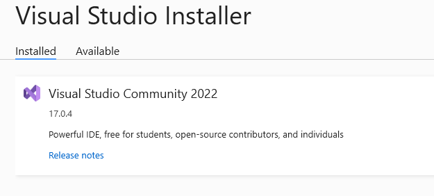
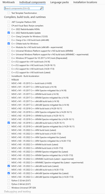
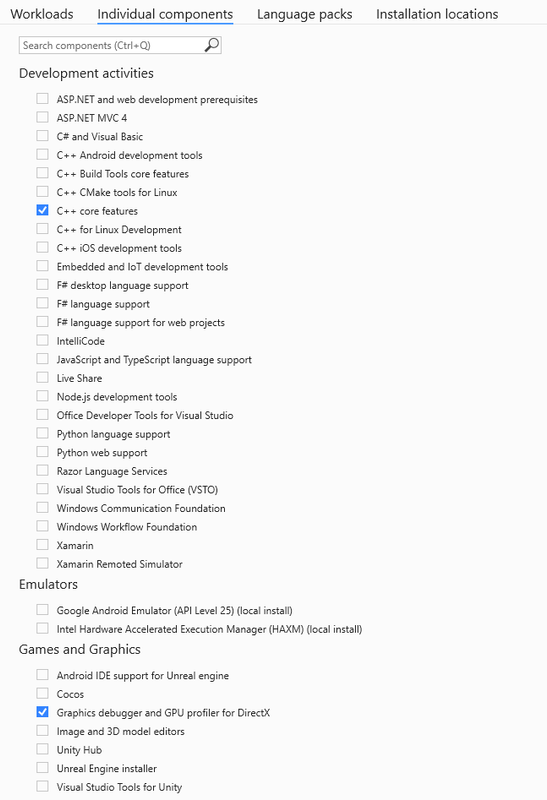
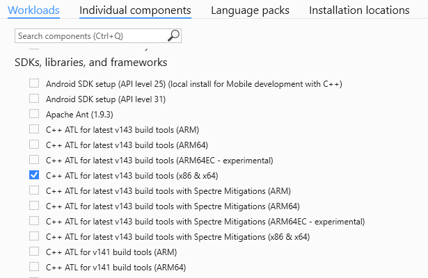
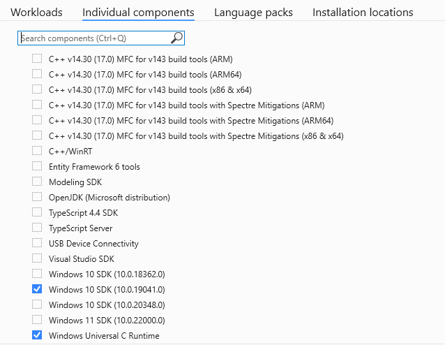
1. Install Visual Studio (this is needed for the C++ compiler): * You need to choose which version of Visual Studio you want, we recommend the 2022 Community version.* Check the next things when installing Visual Studio:
2. Install Qt * Qt installer can be downloaded from here.
* Check the things in the Qt installer as here:
* Try to open QtCreator and load the project. When opening the project for the fisrt time, you may be asked to choose a kit (the compiler for the project). In our case, we have used the MSCV one:
3. Regarding OpenGL: * The library of OpenGL if already in the project. However, if it requires you the file "glext.dll" or the program crashes when running the project on Qt, this dll can be found in the RayTracingSRP folder. Put this dll file in the folder where there are the compiled objects of this project.
User guide: step by step
Note: careful with decimal values (depending on your compiler you may need to change the ',' for '.' and viceversa in the files you want to load).
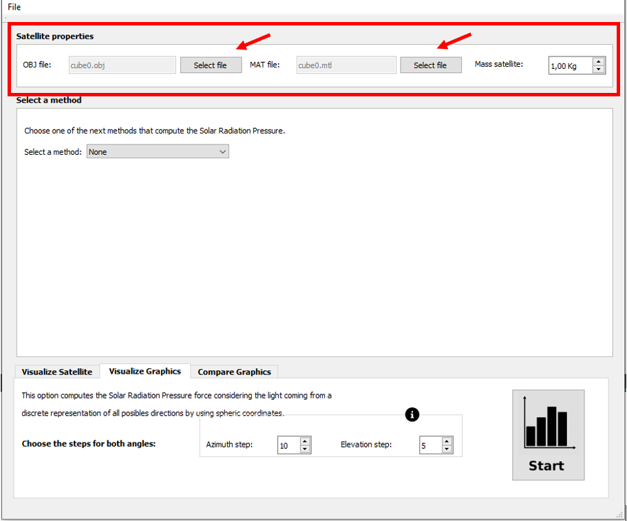
1. Load Spacecraft Model
You need to load the spacecraft model (OBJ file) which is based on CAD model: it contains the list of vertices, faces and normals (optional). Also, you need a MTL file where is described the reflectivy properties of the surface of the spacecraft. In addition, you can set its weight. In the resources/model directory there are examples of this files.
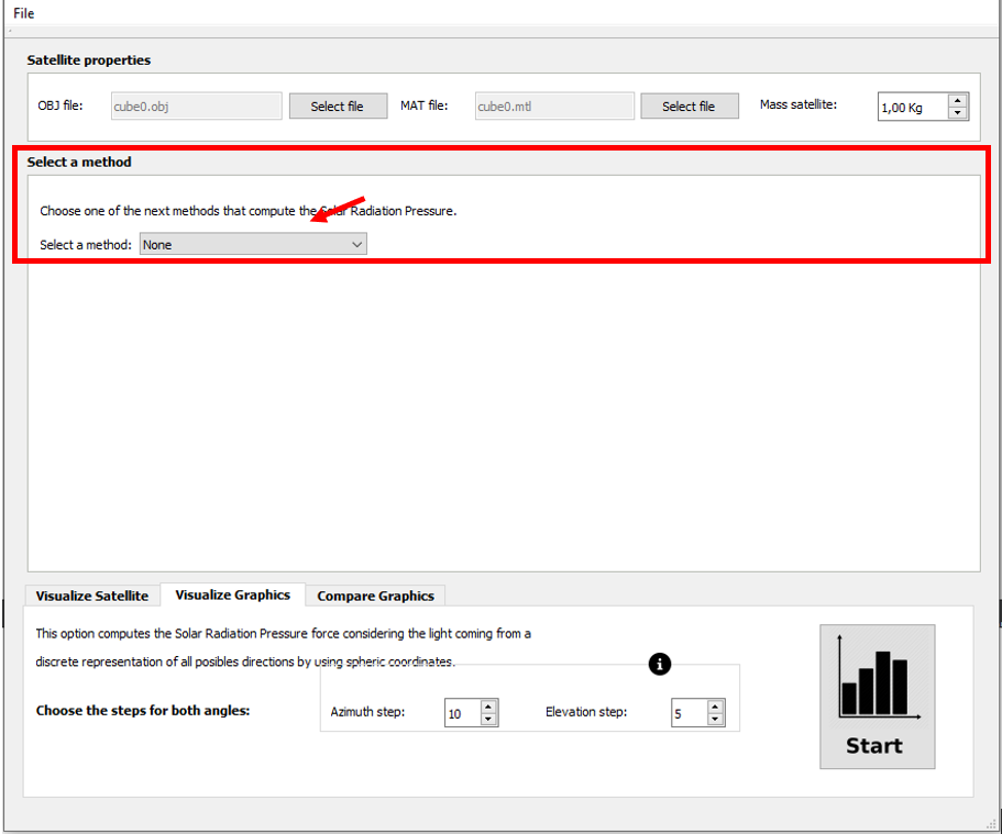
2. Choose a Method to compute SRP Acceleration
You need to choose a method (the model you want to use to approximate the SRP force):
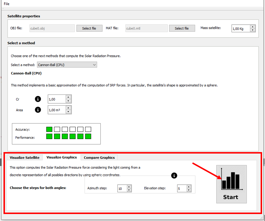
*Cannonball (CPU): considers the shape of the spacecraft to be a sphere. Ypu can set the area of the sphere (A) and the reflectivity property (Cr).
*NPlate (CPU): considers the shape of the spacecraft to be represented as a set of flat plates (you need to load a file that contains the number of plates, and then, for each plate, a new line with the area, specular reflectivity property, diffuse reflectivity property, and normal of the plate; you can see an example in the resources/model directory).
*RayTrace (CPU): for each cell of a grid defined by the number of cells (Nx x Ny) a ray is casted against the triangular mesh of the spacecraft. Then, it is computed the SRP force on the intersected triangle. The user can set the grid and secondary and diffuse rays.
*RayTrace (GPU): Similar to the CPU version, in this case the computation is done in the GPU. The user can set the secondary and diffuse rays. (Nx = Ny = 512 by default).
3. Choose an Action to perform
You need to choose what action you want to do:
* Visualize spacecraft: when the user press the start button in the Visualize Spacecraft tab, it will show a 3D viewer of the spacecraft with its 3 axes and the sunlight direction. Then, the user can set the initial rotation of the spacecraft by interacting with the three sliders. Each one of them corresponds to one of the local axes of the spacecraft.
For example, in the first slider, it appears "X" in red and this indicates that the red line in the 3D viewer correspond to the x axis. The user can also rotate the scene by pressing the right button of the mouse. It will not affect the computation of the SRP accelerations because it is modifying the orientation and position of the observer (camera) and nor the model neither the sunlight direction. And having pressed the left button, the user can zoom in and zoom out.
Also, it allows the user to compute and visualize particular accelerations by rotating the spacecraft after having pressed the ’Start’ button and consequently, interacted with the sliders.
These accelerations that will appear in the 3D scene would have a different colour depending on their magnitudes. It was chosen to use the heat map colours to represent in blue the forces with lower magnitudes and in red the ones with higher magnitudes. Also, in this window it indicates which is the lowest and the highest magnitude among the accelerations that were computed.
* Visualize Graphics: it computes the SRP acceleration considering a set of pairs of azimuth and elevation angles. The user can select the azimuth and the elevation steps (they indicate how many points are used to discretize sample points from a sphere).
if a GPU-based method was selected, another option would be added to this tab and it allows the user to visualize the results obtained from SRP accelerations while the computation of the global accelerations is being done.
If the user pressed the "Start" button, these accelerations would be represented in a window with four 3D viewers showing each one of the components of the acceleration (x, y and z) and also its magnitude (see Fig. 17 and 18). In addition, the user can download the result as a txt file.
* Compare Graphics: this option allows the user to compare the result of two graphics that were previously generated. It is important to have this tool of comparison because it lets the user to compute the difference between two already computed graphics. Also, it shows the mean square error (MSE) and the maximum difference between the points on the charts.
